Kafka Streams – Catching Data In the Act. 1

I have been playing with Kafka on and off lately. It is an excellent addition to the ecosystem of big-data tools where scale with reliability is imperative. I find it intuitive and conceptually simple (the KISS principle) where the focus is squarely on reliability at scale. Unlike the traditional messaging systems that attempt to do many things, Kafka offloads some tasks to the users, where they rightly belong anyway – like consuming messages. Kafka employs the dumb-broker-smart-consumer paradigm whereas the traditional systems do the opposite. In Kafka, the users get full control over the consumption of messages like re-processing older messages if they want to for example, and Kafka gets to focus on message throughput, persistence, parallelism etc…It is a win-win. More importantly it enables Kafka to natively enable complex stream processing capabilities so that https://kafka.apache.org/ now-a-days describes¹ itself as a “distributed streaming platform” rather than a messaging pub-sub system.

The purpose of this post is illustration – we pick a simple, made-up (but intuitive) set of data streams generated by different sensors. Each stream of data on its own is inconclusive in assessing the overall health of the process. They need to be looked at in the aggregate, i.e in conjunction with data from the other sensors in order to compute a health metric for the process. And we will use Kakfka Streams to do just that.

1. Stream Processing

Stream processing allows for catching the data “in the act” – so to speak. This is as opposed to waiting to ingest that data on a back-end platform and then running health queries to check if all went well. If we do find in that case that it did NOT go well – too bad, it has already happened.The best one can do is learn from it and update the processes so it may not repeat. When this is unacceptable, we need the means to analyze the data as it flows so we can either take a remedial action or at least alert – in real-time. Having this means to generate preliminary alerts based on incoming data “as it happens” can be useful before a deep dive later on as needed. Kafka as the data bus has been coupled with tools such as Spark for stream processing. But this adds extra layers & clusters to the platform. If one is not already heavily invested in these other tools for stream processing, Kafka streams would be a natural choice as the data is already being fielded by Kafka anyway. I do see people converting their apps to use Kafka streams on that simple account.

A data stream is an unbounded, ever-increasing set of events, and as such these data streams are routinely obtained in daily life. In many cases there is a need for real-time analysis across multiple streams of data  for critical decision making. For example:

• Health monitors. Often there are multiple monitors measuring different aspects, and they need to be considered together, rather than each on their own.
• Reaction Chambers. Monitoring a reaction chamber for temperature, pressure and concentrations of hazardous gases/liquids is essential for safe operation. Each feature has its own sensor throwing off a stream of data. As the physicochemical processes are coupled, these data streams should be evaluated together to diagnose unsafe conditions.
• Leak Detection. The upstream flow gets split across multiple downstream pipes in a dynamic fashion, as the valves are operated. The total downstream flow should conserve however, else there is a leak.
• Earthquake Sensors. The shear forces during an earthquake distort structures, and the resulting displacement at critical junctions can lead to a complete collapse. If these junctions have been fitted with sensors capable of sending (& still functional during & post the shaking event!), their positional data, engineers can analyze them together to evaluate the overall strain being built up in the structure. We will look at a very simple use case of this in this post.

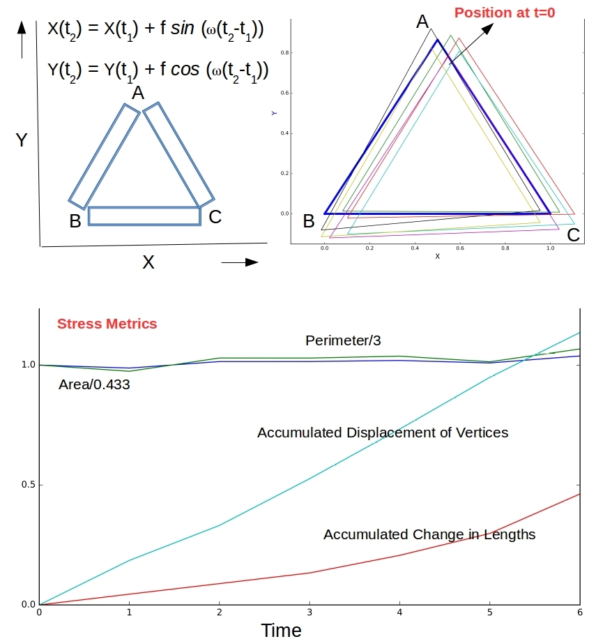
Figure 1. A simulated view of deformation as A, B and C experience somewhat periodic movements. ‘f’ is a random amplitude designed to create noise around the base signal. Cumulative metrics could be better indicators of stress than snapshot metrics

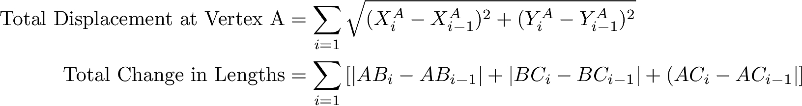
Figure 1 shows 3 metal plates riveted at their ends forming an equilateral triangle with unit sides (Area 0.433 & Perimeter 3.0), on a plane. The sensors at A, B, and C continuously throw off positional data – the X and Y coordinates in a common reference frame. A psuedoperiodic movement with randomized amplitude f is simulated for the three vertices. Movement at the junctions causes stresses in the plates and in the supporting structure. Overall stress metrics with predictive ability can be computed and used for alerting.  With the index and referring to successive measurements we have:

2. Process topology

Converting the above scenario to a topology of data streams & processors is straightforward as shown in Figure 2.

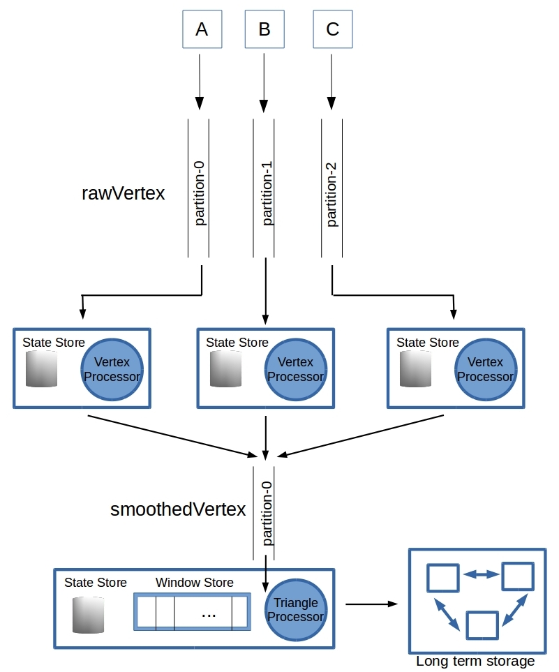
Figure 2. As many source topic-partitions as the number of sensors/vertices. Each processor uses local store to recover state in case of failure. The triangle processor uses a time-binned event store to detect simultaneity.

The core elements of the topology are as follows.

1. Topics. Two topics – “rawVertex” and “smoothedVertex”. The topic rawVertex with 3 partitions and smoothedVertex with 1 partition.
2. Source Producers. Three producers A, B, and C – each generating positional data to a distinct partition of the topic rawVertex. Hence, as many partitions for the rawVertex topic as the number of vertices being followed – here equal to 3. The value of the message is the measurement object consisting of the current coordinates, the timestamp, a count number etc…
3. Vertex Processor. A stream task attached to a partition of rawVertex topic sees all the positional data for that vertex and in the same order as it has been produced, ignoring data loss, data delay issues prior to the data making it to the partition. These issues are mitigated in the Kafka implementation of the producer by having no more than 1 in-flight record at a time and no retries. That is nice because then the vertex processor can confidently compute time averages locally as it receives the measurements. The sensors are noisy so the raw data stream is time-averaged over short periods (short enough to not mask any trends however) producing messages for the smoothedVertex topic.
4. Vertex State Store. The vertex processor in #3 above will use a local persistent key-value store. It will have the most recent smoothed measurement for that vertex, along with any locally computable metrics such as the total displacement of the vertex. In case the stream thread crashes and is restarted, it will get the most current state for this vertex from this local store.
5. Triangle Processor. This is where the merged data streams from he individual vertex processors are used to identify a ‘triangle’ as a function of time. We compute the various global stress metrics indicated in Figure 1, and make the ‘call’ on whether to alert.
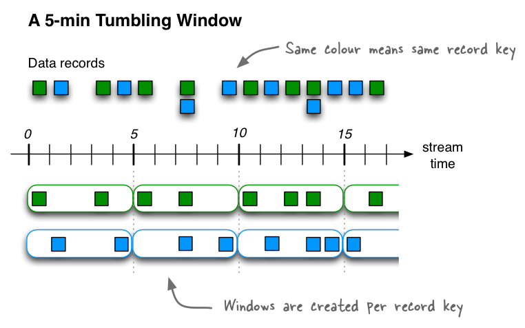
6. Triangle Window Store. In order for a triangle to be identified, we need the coordinates of A, B & C at the same instant in time. The concept of exact simultaneity is problematic when working across streams. Here we employ Kafka’s tumbling windows that bin the smoothedVertex data for A, B & C into time-windows. All measurements that were made (as per the time in the smoothedVertex data) during a window time-period, fall into that bin. The size of this time-window should be small enough so we can take it as an instant in time (perhaps the center of the window), but big enough that at least few items of smoothedVertex data from each of the vertex processors for A, B, & C can land in that bin. See the schematic below (for full disclosure – the diagram 2A is essentially a reproduction of this image put up by good folks at Confluent!)
   

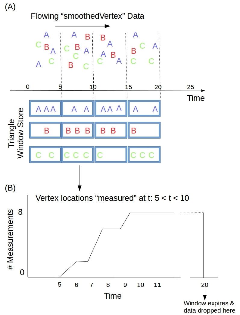
   Figure2. The window state store. (a) Flowing data is binned into time windows. The ‘measurement time’ of a data point determines which bin it ends up in. This means that the points in a bin can be used to approximately identify the triangle at a ‘point’ in time – perhaps the midpoint of the bin (b) A  window starts out empty, accumulates data as measurements flow in from the smoothedVertex topic. It reaches a maximum and stays there until the window is dropped after the retention time is reached. The retention time is chosen so that we can detect the plateauing of the data count in the bin, and also have enough time to compute stress metrics for the triangle.

7. Triangle State Store. The triangle processor needs a persistent state store as well to account for failure & restart. When a window plateaus we compute the triangle state (current vertex locations, the lengths of the sides, perimeter, area, and other stress metrics…).
8. Long Term Storage. Periodically the triangle processor dumps the state store data to long term storage like Elasticsearch for deeper analytics.

3. Data model – Avro schemas

Disk is the life-blood of Kafka. Reading from and writing to disk is its bread & butter. Data is written to disk and pulled from disk as it moves on down from the source topics via intermediate topics to its long term storage. So the serialization of our raw & smoothed vertex ‘objects’ as they are written to disk and their deserialization as they are read back into the code is important. Thankfully we have the Avro schemas to define the data structures in and Kafka (via Confluent) providing builtin support for serialization & deserialization of avro objects.

3.1 RawVertex.avsc

The raw measurement from the sensor at a vertex is the value for the topic “rawVertex”. The key for the topic is the name of the sensor (“A” or “B” or “C”) of course. and are the instantaneous values for the vertex location.

3.2 SmoothedVertex.avsc

The vertex processor smooths the incoming measurements from rawVertex topic over short periods of time. It saves the latest one to its local store and also pushes it onto the smoothedVertex topic.

 X and Y in these records are the time-averaged coordinates of this vertex/sensor over the period timeStart – timeEnd . The displacement distance of the vertex due to each successive measurement is accumulated in cumulativeDisplacementForThisSensor. If the vertex processor were to crash, and restarted, it has enough information in its local store to continue on from where it left off.

3.3 Triangle.avsc

The triangle processor is where the rubber meets the road. The evolution of the triangle, and the stress metrics are computed and saved to a local store and purged to long term storage periodically. The model for the triangle will have the usual suspects like the vertex locations, sides, area etc…. and the cumulative displacement of vertices over the entire time. On what basis to alert on is not the focus here – we can make it up.

4. Conclusion

The core pieces of the problem and the solution approach have been laid out here. What is left is the implementation and a walk-thru of code snippets as needed to make the points. As this post is already getting a bit long we will take it up in the next installment.

1. Kafka® is used for building real-time data pipelines and streaming apps. It is horizontally scalable, fault-tolerant, wicked fast…