Kafka Streams – Catching Data in the Act. 2: Steady and Unsteady States

I was on vacation with my son at Yosemite over the spring break this past weekend. Early part of the trip was washed out due to rain as they closed the park and we were cooped up in the lodge waiting it out. But we had a patio view of the Merced river and the torrent of water gushing through. Loads of time to break out the laptop and write up the long overdue second installment to the use of Kafka Streams. So here we go.

In the previous post we laid out a monitoring problem and a solution approach with Kafka Streams. Here we go over the design of the experiment and simulate it to convince ourselves that it all works as expected. We start with the overarching timing belt, the pace, and the resiliency concerns that should be accounted for in the design. We want to have an intuitive feel for the rhythm of the operation and know what to expect before we start generating a lot of data.

The objective of this post is to go over the factors we need to consider in the design, understand the capacity of our system, characterize it in terms of operational delays inherent in the system, and plan for failures & recovery. We run a few simulations as we go along to confirm that the results are as per the design.

1. Simulation Design

The apparatus for the experiment to twist the triangle is the laptop. The three producer processes get started at the same time and write the rawVertex data to disk. The stream process pulls the rawVertex data, smooths them over a short contiguous period, writes to various state stores, computes stress metrics and saves to long term storage. That is the big picture.

1.1 The timing belt

Stream operations live and die by time. So first, the operational definition of time in the model is critical as the monitors and/or the stream processors can go down & restarted,  get stuck in expensive calculations, or the network slows down the delivery of messages etc…, even as the wall-clock chugs along uninterrupted. The good folks at Kafka have realized this and allowed for the  concept of Stream Time to be defined as per the needs of the use case.

In our case this would be the time a measurement is made, or a close enough instant in time when all three vertices have a measurement – so we can approximate a snapshot of the triangle (it certainly will not do to define a continuously deforming triangle with the positions of the vertices measured at widely different times). This stream-time will NOT advance if no new measurements emanate from the monitors – perfect!

1.2 The clip

Second, we need to have an intuitive understanding of the operational rhythm so a quick glance at the various metrics in a production scenario at say 4 AM can tell us what may be amiss. This is the clip of the operation – like the number of raw/smoothed measurements, and the number of triangle metrics per unit time that we should be seeing on a production dashboard. This pace of the operation is determined by the rate of rawVertex production at the monitors, the smoothing interval at the VertexProcessor before it produces a smoothedVertex, and the window size (& its retention time) in the TriangleProcessor. A few obvious considerations would be:

• Smoothing interval: The smoothing interval employed by the VertexProcessor should be small enough to not to mask any trends while removing noise. This interval defines the minimum size of the window in the TriangleProcessor.
• Window size: Too big a window size means that the triangle is not close to a snapshot image. Too small a window size may yield zero number of measurements from one or more of the sensors. We need at least one measurement from each sensor/vertex to fall in a window in order to define a triangle.
• Window retention time: Too small a retention time means any late arriving messages will not be used, leading to some windows having zero measurements for a vertex even while the window is about to be dropped – meaning no triangle can be defined for this window period. But too big a retention time means more book keeping, computation,  disk usage, and likely a longer wait for a metric to plateau/saturate.

1.3 Latency and steady/unsteady state operations

Third, we have to take into account the limitations of the apparatus (the laptop as is the case here) at hand, such as latency and contrast between the steady and unsteady operational states.

• Latency: How long does it take for a trend at the monitors to manifest itself as a trend in the stress metrics for the triangle, under a steady state operation? This is the core latency inherent in the system determining how fast we can respond to events.
• Capacity & Resiliency: If the stream processor dies and is restarted, it will pick back up at about the same stream-time as when it went down, as the processor is backed up by persistent state stores (rocksDB). There is no data loss. But, how long does it take for the system to catch up and reach steady state? This is the  capacity & resiliency of the system.

In a steady-state operation, the rate at which the raw vertices are delivered stays about the same. But when the stream processor comes back up after a failure, it can get overloaded with all the backlogged measurements. The VertexProcessor gets too busy to spare time to forward the smoothed measurements to the next stage. The punctuate/forward operation is best effort meaning if the processor is otherwise busy, the punctuate operation may be delayed or clubbed with the next punctuate op. If the processor has been down for an extended period of time, one can see large delays in producing the first smoothed vertices after a restart.

2. The Steady State

With the above discussion in mind, we proceed with the simulation in steady state.

• 1 raw vertex per second: The producers sleep for 1 second after producing a message to the rawVertex topic. So there could be no more than 60 raw measurements delivered to each partition in a minute.
• 5 smoothed vertices per minute: Vertex processor punctuates (ideally!) the forward operation every 12 seconds. That is, the vertex processor keeps a running average of the X and Y coordinate values for 12 seconds, and then forwards those averages to the smoothedVertex topic before starting a new smoothing batch. So in ideal conditions we should see no more than 12 raw measurements (as the monitors are producing 1 measurement a second) in each average, with 5 such averages being produced per minute. The three VertexProcessors together then pump 15 smoothed measurements to the smoothedVertex topic in a minute.
• 1 triangle per minute: The window store employs 1 minute windows so we get a triangle snapshot for every minute of stream-time (& real-time in a steady state operation)  that we can alert on if needed.
• 3 hrs of window retention: Each window lives for 3-hrs of stream-time before it is disposed off. In a steady state operation, 3-hrs is plenty of time to saturate a window with all the measurements it can ever get.

Running the simulation for over 12 hours and capturing the beat for verification on Elasticsearch+Kibana, we see that our design holds up with respect to the rate of production of messages & metrics.

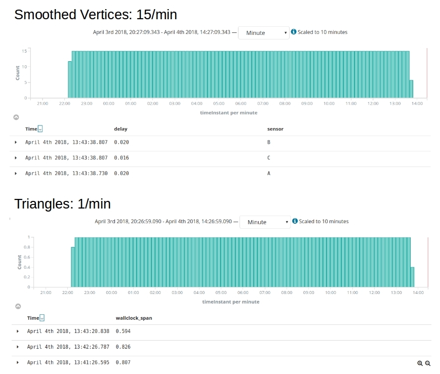
Figure 1. Steady State Operation. 1 rawVertex/min & 12 seconds of smoothing. So 3 (vertices) x 60/12 = 15/min smoothed vertices. 1 min window size means one triangle per minute. As expected from the design.

But what about latency? Figure 2a below shows the latency of smoothed vertex messages in the stream process.

• There is essentially no delay (a few milliseconds may be?) in receiving a raw measurement from the producer (not shown in Figure 2)
• Travel-Time: Travel-time is the elapsed wall-clock time it takes for smoothed vertex message to make its way from the VertexProcessor where it is emitted, to the TriangleProcessor. On the average it takes 1.6 seconds (Figure 2A). Not sure if 1.6 seconds on a laptop is considered too long. Probably attributable to all the push-pull ops at the disk, and the fact that the laptop was loaded all through the simulation.
• Saturation-Time: Saturation-time is the elapsed walll-clock time between the latest arriving smoothed vertex into a window, and the earliest arriving one. On the average, a typical window saturates in about 49 seconds (Figure 2B)! That is fantastic, as it means we can cut the window retention time way back from what we chose as 3 hrs in the design. But we will have to see how a restart scenario looks like before we do that.
  

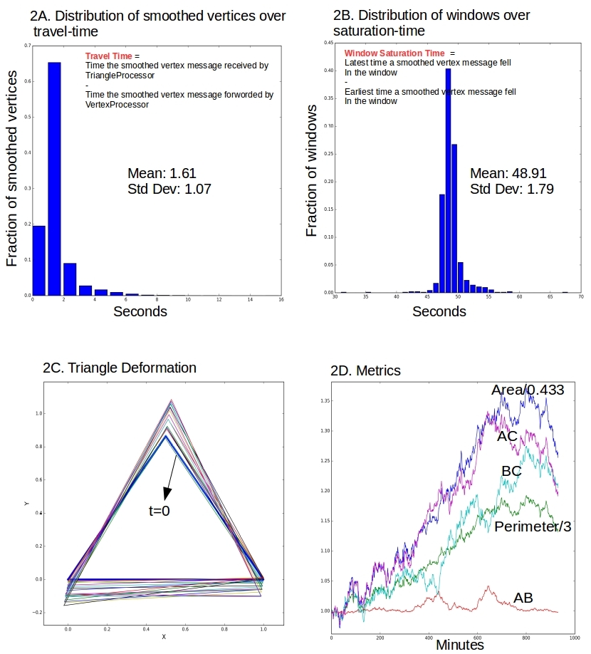
  Figure 2. Steady state operation. 2A shows the spread of the “travel-time” or “stream-delay” for a smoothed vertex messages to go from VertexProcessor to TriangleProcessor. 2B shows the spread of the wall-clock elapsed time between the earliest and latest arriving messages in to a window, that is he “saturation-time”. 2C & 2D show the deforming triangle and some metrics with time.

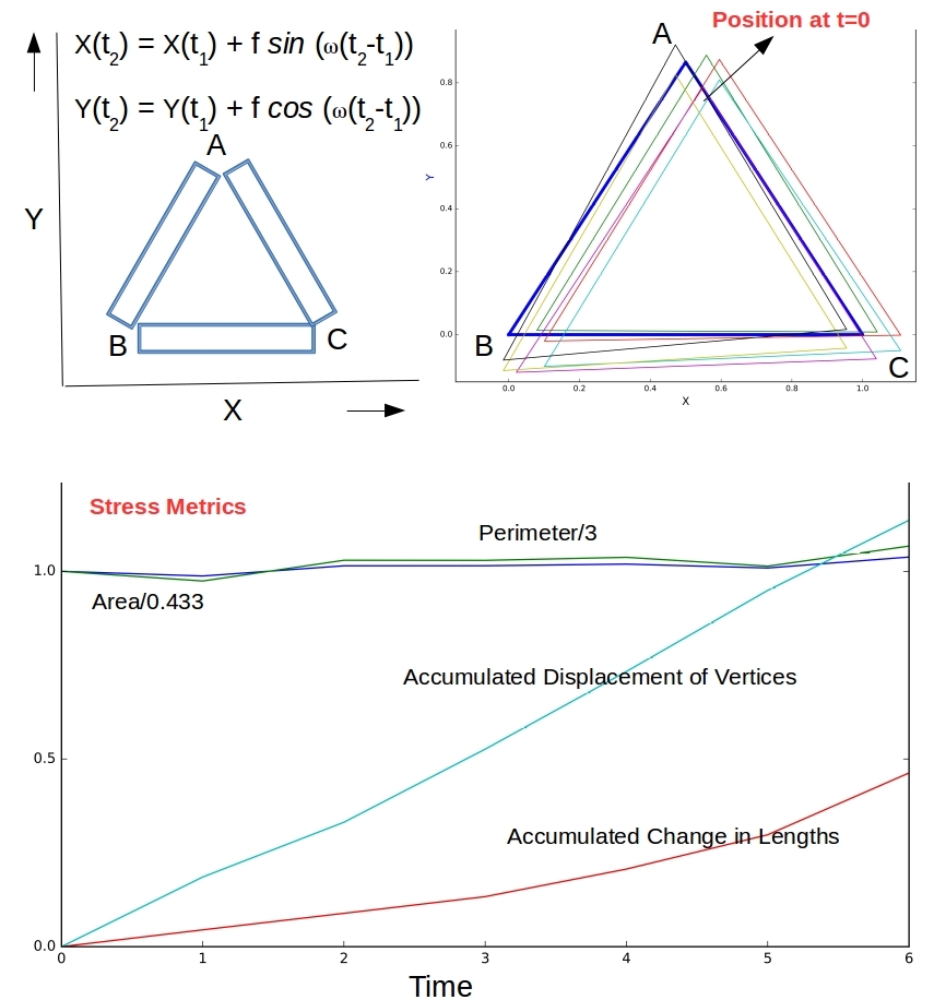
• Figures 2C & 2D show the metrics from this run. They are quite similar to pictures we produced via analytical means in the earlier post. Makes sense as we apply the same perturbation to the vertices.

A snapshot of the current offsets (obtained with Kafka-Utils) during the steady state shows that the processing is humming along nicely with just a few measurements on the disk waiting to be processed (see Lines 7, 14, 20 & 26 below). This is the desired behavior and if anything it shows that we may be able to increase the production rate and the laptop may still be able to stay current. But we will see in the next section that we do need this extra processing capacity to quickly lead us out of an unsteady state to steady state.

3. The Unsteady State

Unsteady state results when the stream processor has a backlog of measurements to process. This causes some hiccups in the processing rhythm of the operation until it all stabilizes once more.  We know for a fact that it will stabilize given enough time – because of our conservative design parameters. Our conclusion from Section 2 is that we have excess capacity in stream process that will eat into the backlog and eventually catching up to work on the currently produced measurements.

We simulate two periods of unsteady state.. We start the producers, build up data in the rawVertex partitions a bit and then start the stream processing. This gives rise to the first period of unsteady state. After achieving the steady state and running for a bit, we kill the stream process, wait for several hours and restart it to give the second period of unsteady state. For example the state of the offsets just before the second period of unsteady state is as follows. There is no backlog (line # 8 below) in the smoothedVertex as expected. But we have built up a significant backlog to be processed in the raw vertices (lines # 15, 21, 27 below).

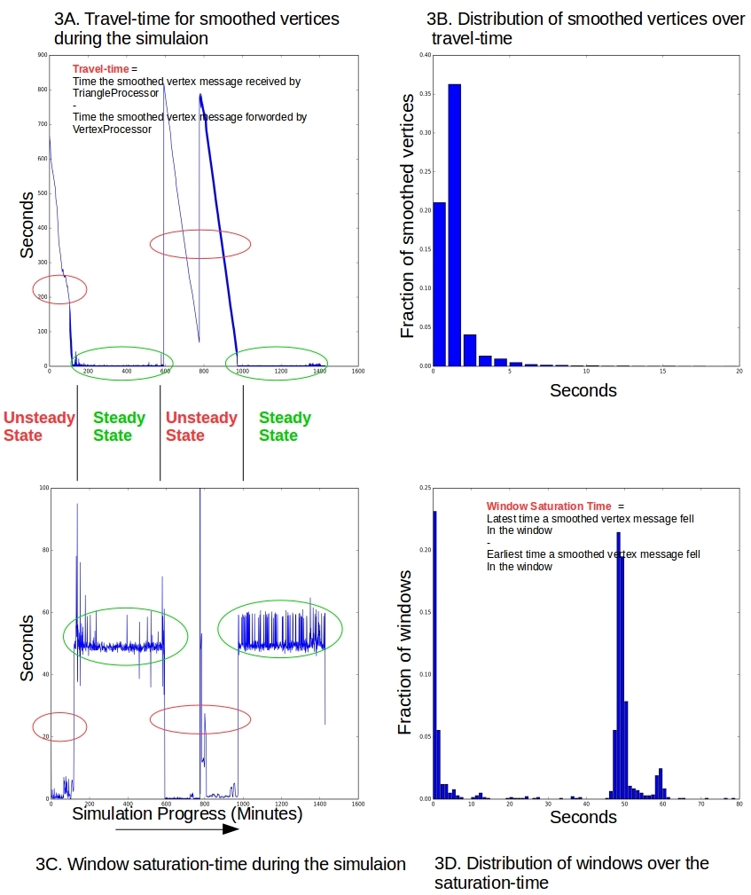
Figure 3. Unsteady & steady states. 3A: The apparent “travel-time” for a smoothed vertex to make its way from the VertexProcessor to the TriangleProcessor is larger during unsteady-states. It approaches its steady-state value as the stream processor catches up with the backlogged messages. 3B: Smaller fraction (57%) of overall smoothed vertices have less than 2 seconds of travel-time compared to the steady-state-only operation (85% see Figure 2A). 3C: Windows saturate right away during unsteady-state as a burst of smoothed vertices unload onto the TriangleProcessor. As the stream processor catches up, the natural rhythm reasserts itself and the saturation-time goes back up to a minute as in the steady state. 3D: Window saturation-time has a bi-modal nature. The first mode corresponds to the steady-state value, and other near zero, reflecting the burst of smoothed vertices into the TriangleProcessor.

The simulation results in Figure 3 bear out many of the assertions we have been making about the steady and unsteady states.

1. Delays in receiving the smoothed vertices. Figure 3A plots the wall-clock delay in receiving smoothed vertices at the TriangleProcessor after they are forwarded by the VertexProcessor as the simulation continues. The unsteady states are characterized by sharply higher initial delays that decay with time as the operation marches to a steady state with smaller delays in single digits. These larger delays during the unsteady state  influence the overall distribution shown in Figure 3B. Only about 57% of messages have a delay of less than 2 seconds in this steady+unsteady simulation, compared to about 84% of messages in the stead-state only simulation in Figure 2A.
2. A torrent of triangle metrics. Figures 3A and 3C make for an interesting pair. During the unsteady state a large number of punctuate operations are clubbed together as one in the VertexProcessor. This is why we observed the delays noted in item #1 above. But this exact behavior dumps a whole bunch of smoothed vertices in one shot to the TriangleProcessor, and the time-windows in the window-store saturate right away. This means that there is not much wall-clock time-gap between the earliest arriving message in a window and the latest arriving one. This gap dives to zero during the unsteady state.
3. A bi-modal distribution for window saturation-time This is shown in Figure 3D. During each period of unsteady state, the time taken to saturate a window in the window-store, is near zero and recovers to its steady state value that we know to be under a minute from Figure 2B. This sets up an approximate bi-modal for the distribution of window saturation-time.

4. Conclusions

We spent a good bit of time looking into the dynamics, the ebb & flow of messages under different conditions. Simulations such as these to establish the operational metrics for normal & failure conditions are essential to develop insight into the system. We will get to the actual code & mechanics under these simulations in the next installment.