Quotes. Lexical Fuzziness

The road to ‘Computational Linguistics Nirvana’ is littered with thesis upon thesis, stacks of journal papers, and volumes of conference proceedings… so one can get lost in a hurry. Whole programs dedicated to computational linguistics have made great advances over the years enabling the Siris and Cortanas of our time. We are unlikely to make any fundamental contributions to that body of knowledge in this blog. So we take Covey’s advice – ‘Start with the End in Mind‘ and define our rather less ambitious objective. Flagging exact duplicates from our quotes as we did in the previous post was easy. Now we get down to the hard work of flagging quotes that are ‘essentially the same’.  It is very important that we spell out exactly what we mean by ‘essentially the same’ in the context of this blog.

1. Objective

Let us look at the model quote below (attributed to Albert Einstein) in the first column, and its variants in the second column. The second rendition that is struck out is not a real one but made up to illustrate the limits of similarity approaches – especially when we are talking about quotes. With most quotes, there are usually two meanings. The ‘true import’ arises from a context that cannot readily be built from the words used, whereas the ‘apparent import’ is conveyed by the words.  A person reading these quotes will readily understand the ‘true import’ of the model quote and flags the ‘made up’ quote as NOT similar. But we have no practical way to teach the ‘true import’ of the quote to the computer so we steer completely clear of this level of similarity – can’t do it.

Model	Variants	True Import
"I know not with what weapons World War III will be fought, but World War IV will be fought with sticks and stones."	1 "I don't know how man will fight World War III, but I do know how they will fight World War IV with sticks and stones." 2 "I don't know how to fight with sticks and stones"	Our modern weaponry can obliterate human civilization, so avoid wars.

Here we rely on the various metrics that we can compute from the characters & their order, words – their order,  part-of-speech, frequency etc…between the model quote and its variants. This is ‘Lexical Similarity’. Applying this we will correctly flag the variant 1 as similar. That is nice, but we will incorrectly flag variant 2 as similar, and the ‘true import’ as dissimilar! That is the nature of this beast unfortunately! But not all is lost however, as the data is in our favor. Bulk of the ‘near dupe’  quotes in our repo are like variant 1. If we have a way to flag them correctly, we will catch over 90% of our near dupes. With a bit of human oversight we can actually rid the repo of all near dupes.

So we aim to come up with a workable procedure that employs lexical measures to flag fuzzily similar quotes in our rather large repo of quotes (few hundreds of thousands). A procedure that a generic quotation web site can perhaps put in place as a quality measure for example. That in essence is our objective.

There is a slightly more nuanced type of similarity measure called ‘Semantic Similarity‘ that builds a metric out of how similar in ‘meaning’ the words are in the two quotes, so it can work around synonyms to some extent.  My experiments with semantic similarity have been less than fruitful (too noisy, too many false positives, and computationally intensive as well) for de-fuzzing a quote repo but it holds promise for clustering and such that we will look at in a future article.

2. Lexical Similarity Measures

Wikipedia does a great job of reviewing a variety of text similarity measures. There are two types of text similarity measures in general – lexical & semantic as we just mentioned. Lexical similarity that we focus on here, can be character or word/token based. I played with several lexical measures & their variations to see what may be a practical way to detect fuzzily similar quotes as we defined earlier. Here are some  imprecise takeaways:

• Levenshtein, LCS (Largest Common Subsequence), Jaro etc… are examples of character based measures between two strings.
  1. Levenshtein and Jaro are useful when differently spelled words are the issue between otherwise identical quotes.
  2. LCS is perfect when we suspect that the shorter of the two quotes is for the most part embedded in the other longer quote. We compute LCS as:
     
     LCS

     LCS = [Length of the largest common substring] / [Length of the shorter quote]

     1	LCS = [Length of the largest common substring] / [Length of the shorter quote]

• Jaccard, Cosine etc… are examples of word/token based measures. These measures do not care for word order, but just their presence/frequency. If two strings do not share any common words, these measures give a value of 0.
  1. Jaccard is a measure of common words between the two strings. A value of 1 implies a high degree of confidence in similarity (but alas, they could be in different order – but again how likely is that!).
     
     Jaccard

     Jaccard = [Number of Common Words]/[Total Number of Unique Words]

     1	Jaccard = [Number of Common Words]/[Total Number of Unique Words]

  2. Cosine similarity turns each string into a vector (each element representing the number of occurrences of a term for example) and computes the dot product of the two vectors as a measure of similarity between the two strings.

Consider for example the two quotes A & B attributed to Yogi Berra.

A = Baseball is 90 percent mental and the other half is physical.

B = Baseball is 90 percent mental. The other half is physical.

The common piece ‘Baseball is 90 percent mental’ is 50% of the shorter quote B. Also, A & B  share 9 out of 10 total unique words. The unique words represent the dimensions of the vector space [‘is’,’the’,’baseball’,’and’,’90’,’percent’,’other’,’physical’,’half’,’mental’]. In this vector space A is represented by [2,1,1,1,1,1,1,1,1,1] and B by [2,1,1,0,1,1,1,1,1,1]. The numbers here are the number of times that specific word appears in that quote/string. We now get the measures as:

Lucene’s implementation of MLT (More Like This)  employs cosine similarity in conjunction with a corpus of documents it searches against. It prepares tf-idf (The number of times a term occurs in a quote X inverse of how frequent that term is in the overall corpus of quotes) weighted vectors of every quote in its index and the MLT algorithm (speaking imprecisely) simply returns those quotes with the highest cosine similarity measures against the model quote vector. As it turns out this will be our primary workhorse.

3. The Approach

We employ a combination of some of the above measures, and take advantage of what we  know about the nature of quotes.

3.1 Part of Speech Tagging

Quotes that are similar ‘typically’ feature the same nouns, adjectives and even verbs. Purging the quotes of all other parts of speech and punctuation can help amplify the signal when measuring word/token based similarity. Here is a snippet of Python code that removes some common words (same as what Lucene uses to be consistent with Solr MLT) and applies NLTK. One can apply stemming, but it is a double-edged sword. The most I would recommend is removing the ‘s’ at the end.

This transforms quotes in the above table  to

Model	Variants
"know weapons world war iii fought world war iv fought sticks stones"	"don't know man fight world war iii do know fight world war iv sticks stones" "don't know fight sticks stones" "modern weaponry obliterate human civilization avoid wars"

3.2 More Like This Handler

The number of similar quotes for a given model quote is usually just a handful – a small, small fraction of the overall repo size. So we need an efficient first cut that eliminates a whole swath of them from consideration. Solr MLT is blazing fast and we get the ‘potentially similar’ quotes ordered by a score. We process the quotes as above (removing all except Nouns, Verbs, & Adjectives)  and index them into Solr with termVectors, simple tokenization, followed by lower casing and filtering to remove the possessive ‘s’.

An MLT handler ‘/findSimilar’  is configured to return the similar quotes, given a model quote.

Setting ‘mintf’ (Minimum Term Frequency) to 1 is important in our case, as the quotes are short pieces of text and a term may not occur more than once in the quote. Likewise setting ‘mindf’ (Minimum Document Frequency) to 2 allows us to cover the case when a special term occurs in just 2 quotes and those two happen to be similar. To get the similar quotes ordered by a score, we fire http://localhost:8983/solr/quotes/findSimilar?q=id:_THE_ID_OF_MODEL_QUOTE_IN_SOLR_INDEX

3.3 Constrain Matches by Auxiliary Info

If the model quote is X characters long, it is ‘unlikely’ that a similar quote could be 10X long or only X/10 long. So we can remove from consideration quotes whose length does not fall within a band around the model quote’s length. To be cautious, we use a factor of 5 for the length, and let Solr filter out too short/long quotes. Also, it is not very likely that different authors would have come up with lexically similar quotes. We can apply both filters and update our MLT query as:

http://localhost:8983/solr/quotes/findSimilar?q=id:_THE_ID_OF_MODEL_QUOTE_IN_SOLR_INDEX&fq=author:_MODEL_QUOTE_AUTHOR&fq=quoteWords:[_MODEL_QUOTE_WORDS_/10 TO _MODEL_QUOTE_WORDS_*10]

As an aside, we can modify the above query to identify lexically similar quotes that have been incorrectly/differently attributed… by requiring that the author be NOT the same as the model quote’s author. That can trigger an action to be taken later to clean up the data. We shall not pursue this in this post.

At this point we have a set of quotes that are candidates for being lexically similar to the model quote. Note that these are only ‘candidates’ – no guarantees. MLT will simply return the  matches in the order of decreasing similarity – but even the top match ‘could’ be quite dissimilar if there are no lexically similar quotes to begin with in our repo.

3.4 Compute Distance Measures

We now compute the LCS, Jaccard, Jaro etc… distance measures between the model quote and each of the top 20 (or less) potentially similar quotes we got in 3.3. The number ’20’ is arbitrary but covers the worst case scenarios. I have yet to come across twenty different renditions of the same quote. Now comes the hard part though  –  there is no magic formula that combines these measures, with the MLT score in 3.3 in a way that always correctly flags these potentials. There just cannot be a formula of course as we can always come up with a similar quote that will break it – that is the reality. So like any good data scientist we turn to statistics when reason fails!

4. Results

First we need to generate a ‘human curated’ training data set. I took a set of 20 model quotes, chosen for short/long  lengths, having multiple sentences, etc… I  collected the MLT suggestions for each as in 3.3 and computed the various distance measures between model & each of its suggestions. That was good a 400 point data set. The metrics for one such popular model quote by Conan Doyle are in the able below.  Because MLT scores cannot be compared across queries, we normalize it by dividing with the score for the model quote. ‘N-MLT’ stands for this normalized MLT score that falls off from 1 as we move down the table. The suggestions in ‘green‘ are clearly similar so I give them a similarity score of 1. The ones below in ‘red‘ get a similarity score of 0. This binary classification is done ‘manually’ of course – this is the training part.

Sim?	Quote	MLT	N-MLT	Jaccard	LCS	Jaro
	Once you eliminate the impossible, whatever remains, no matter how improbable, must be the truth.	14.032	1	1	1	1
1	When you have eliminated all which is impossible, then whatever remains, however improbable, must be the truth.	4.963	0.354	0.444	0.327	0.775
1	How often have I said to you that when you have eliminated the impossible, whatever remains, however improbable, must be the truth?	4.135	0.295	0.4	0.327	0.729
1	When you have eliminated the impossible, whatever remains, however improbable, must be the truth. It is stupidity rather than courage to refuse to recognize danger when it is close upon you.	3.308	0.236	0.286	0.327	0.67
1	It is an old maxim of mine that when you have excluded the impossible, whatever remains, however improbable, must be the truth.	2.536	0.181	0.333	0.327	0.693
1	Eliminate all other factors, and the one which remains must be the truth.	1.806	0.129	0.375	0.27	0.728
0	Any truth is better than indefinite doubt.	0.132	0.009	0.111	0.207	0.516
0	It is, I admit, mere imagination; but how often is imagination the mother of truth?	0.115	0.008	0.111	0.15	0.668

For each of our distance measures we generate two score distributions. One for the set of quotes we marked as similar and the other for those we marked as dissimilar. The point is that if the two distributions are disjoint we have a great indicator. The more the overlap and noise, the less useful that measure is in picking apart similar Vs dissimilar quotes. The ‘red‘ histograms below give the score distribution for dissimilar quotes, and ‘green‘ for similar quotes.

Normalized MLT

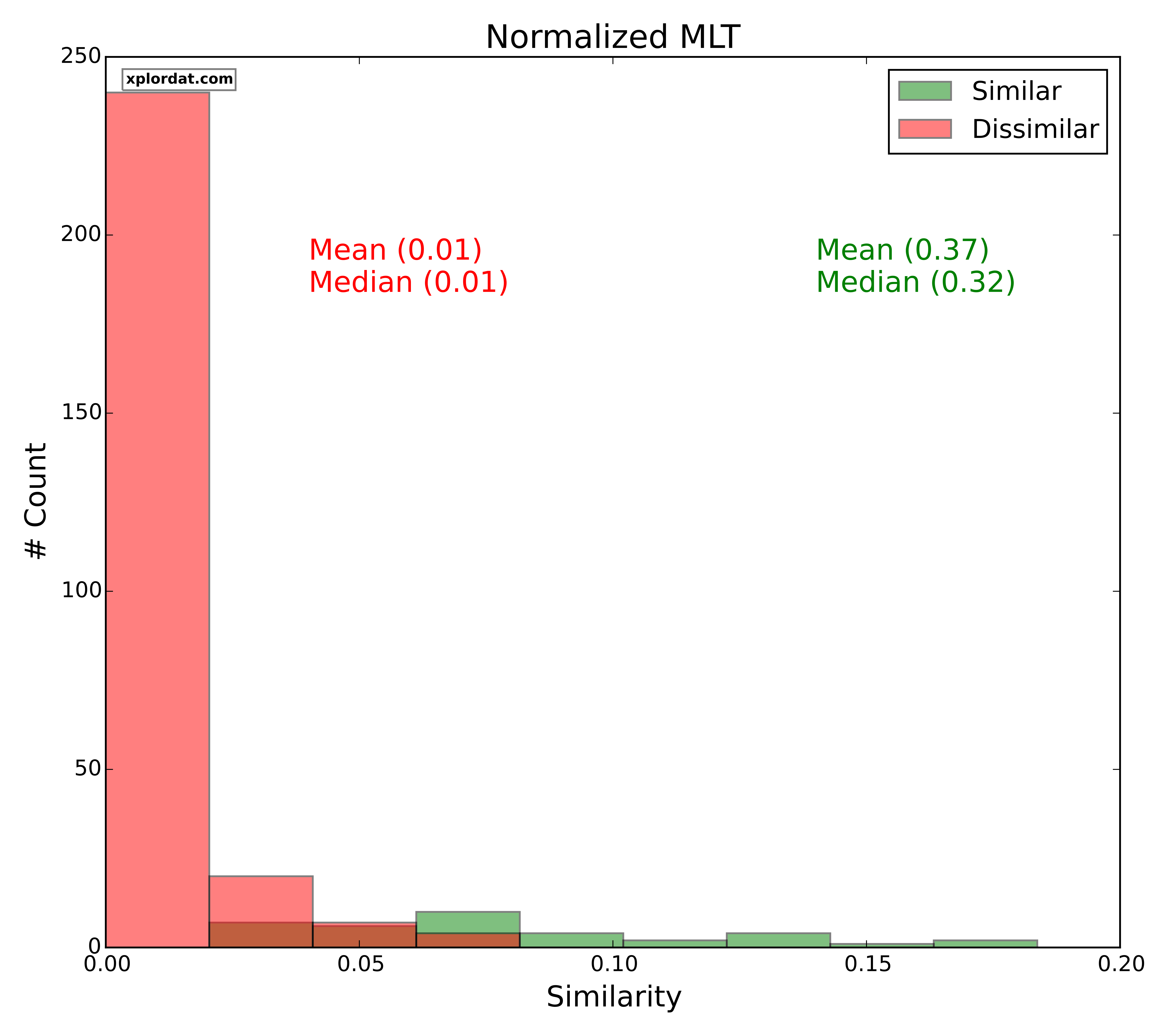
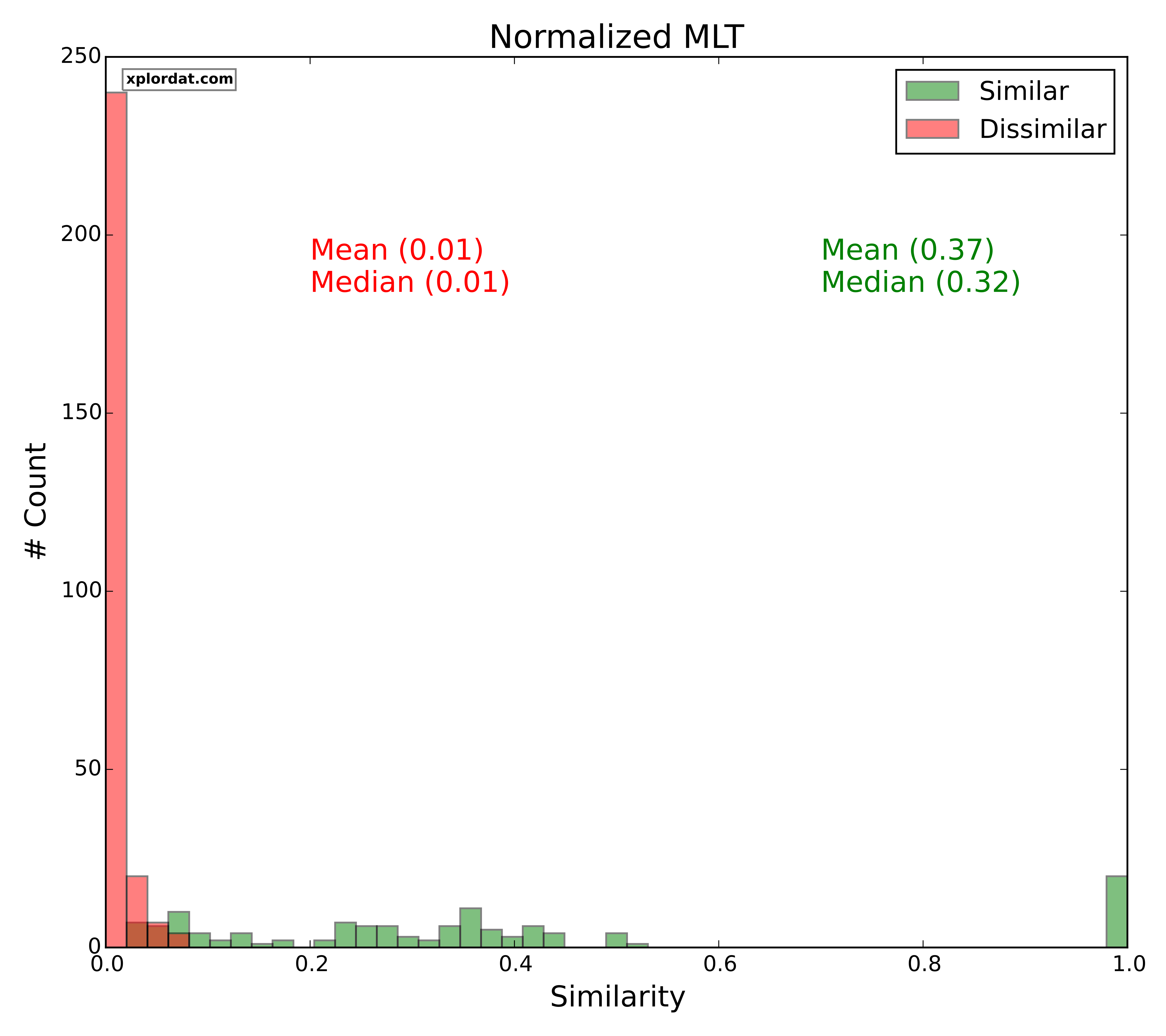
• Normalized MLT > 0.2 => Lexically Similar

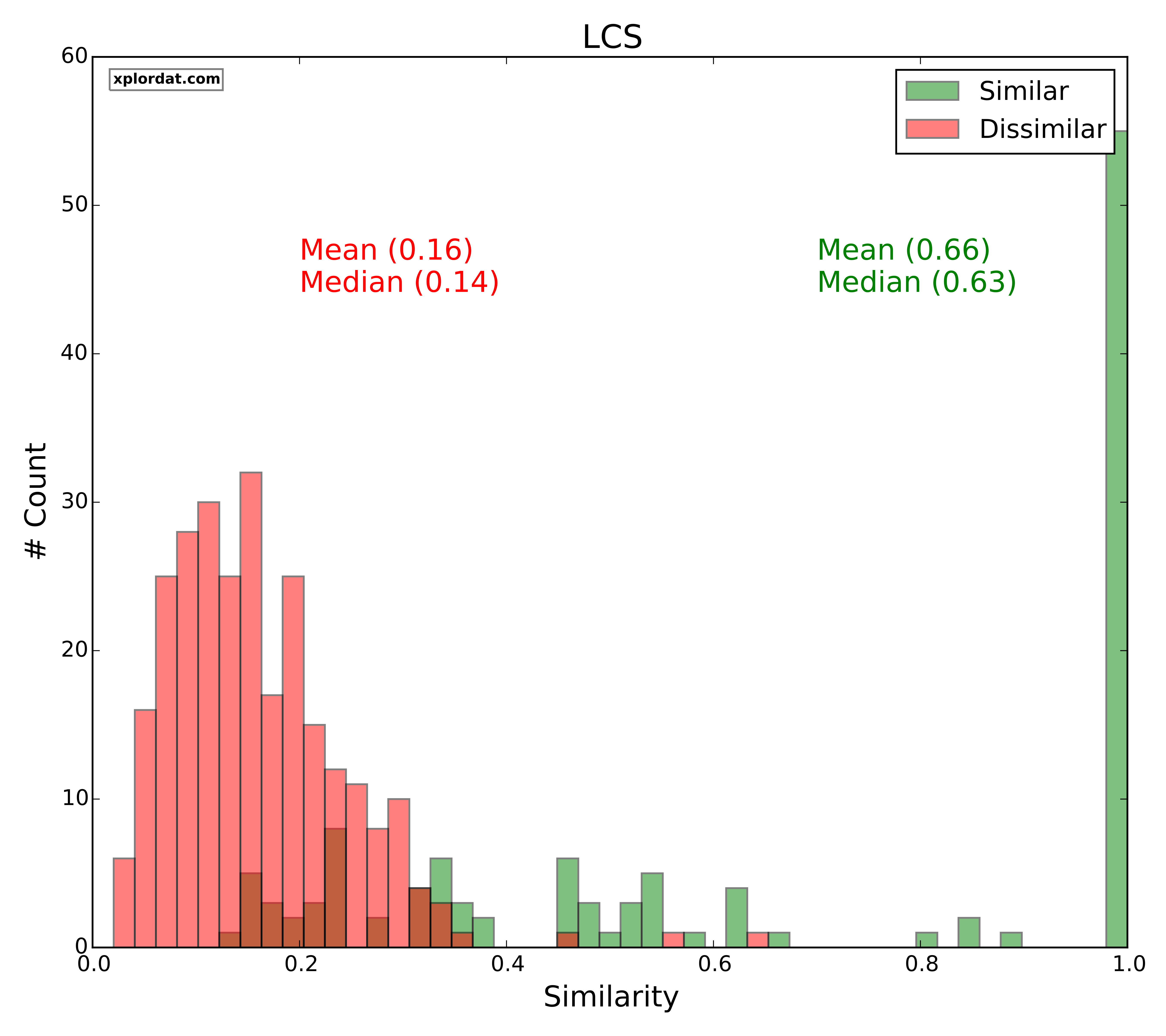
Jaccard, LCS

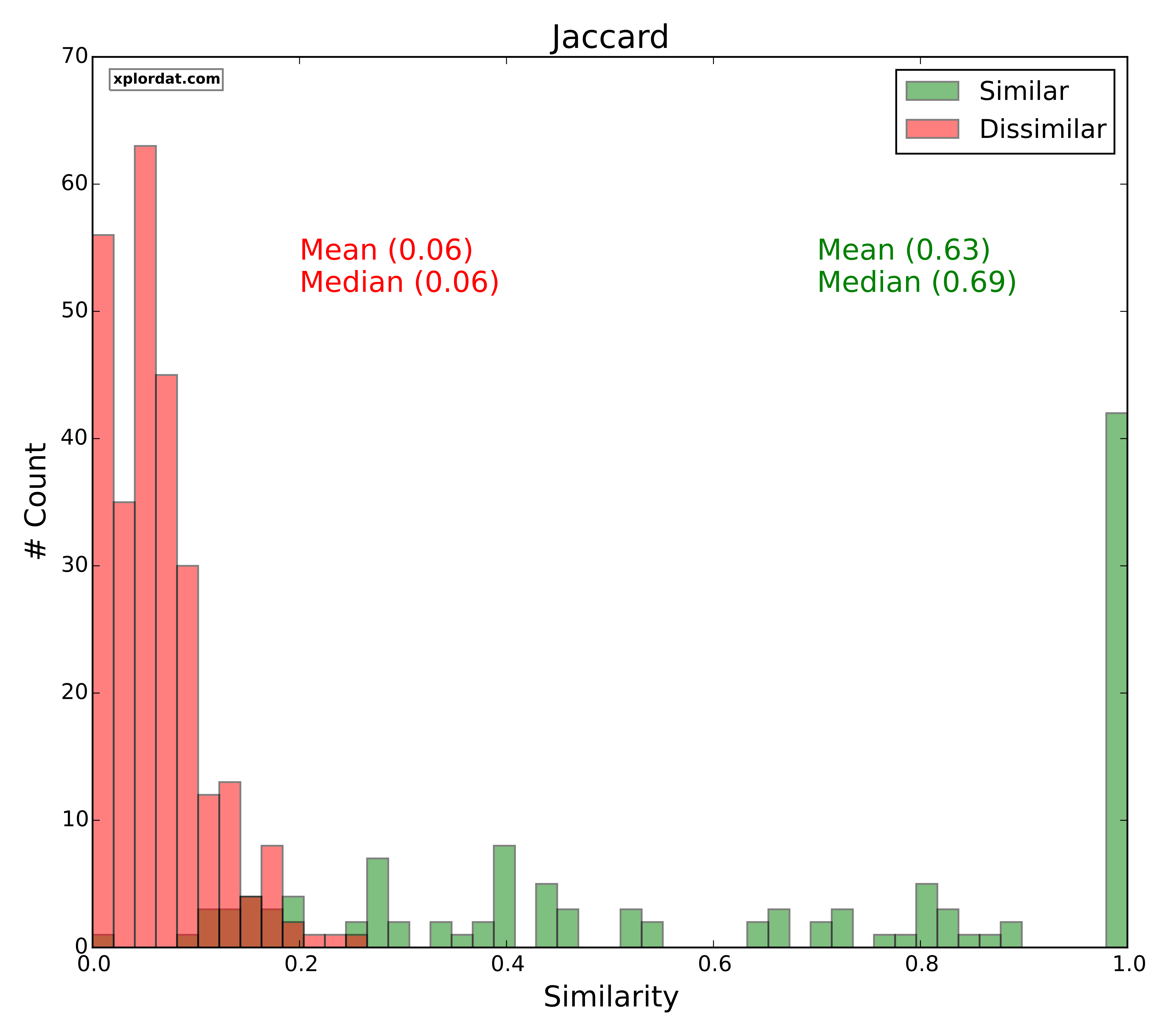
• Jaccard ratio  > 0.3 => Lexically Similar
• LCS measure > 0.5 => Lexically Similar

Jaro, Difflib Sequence Ratio

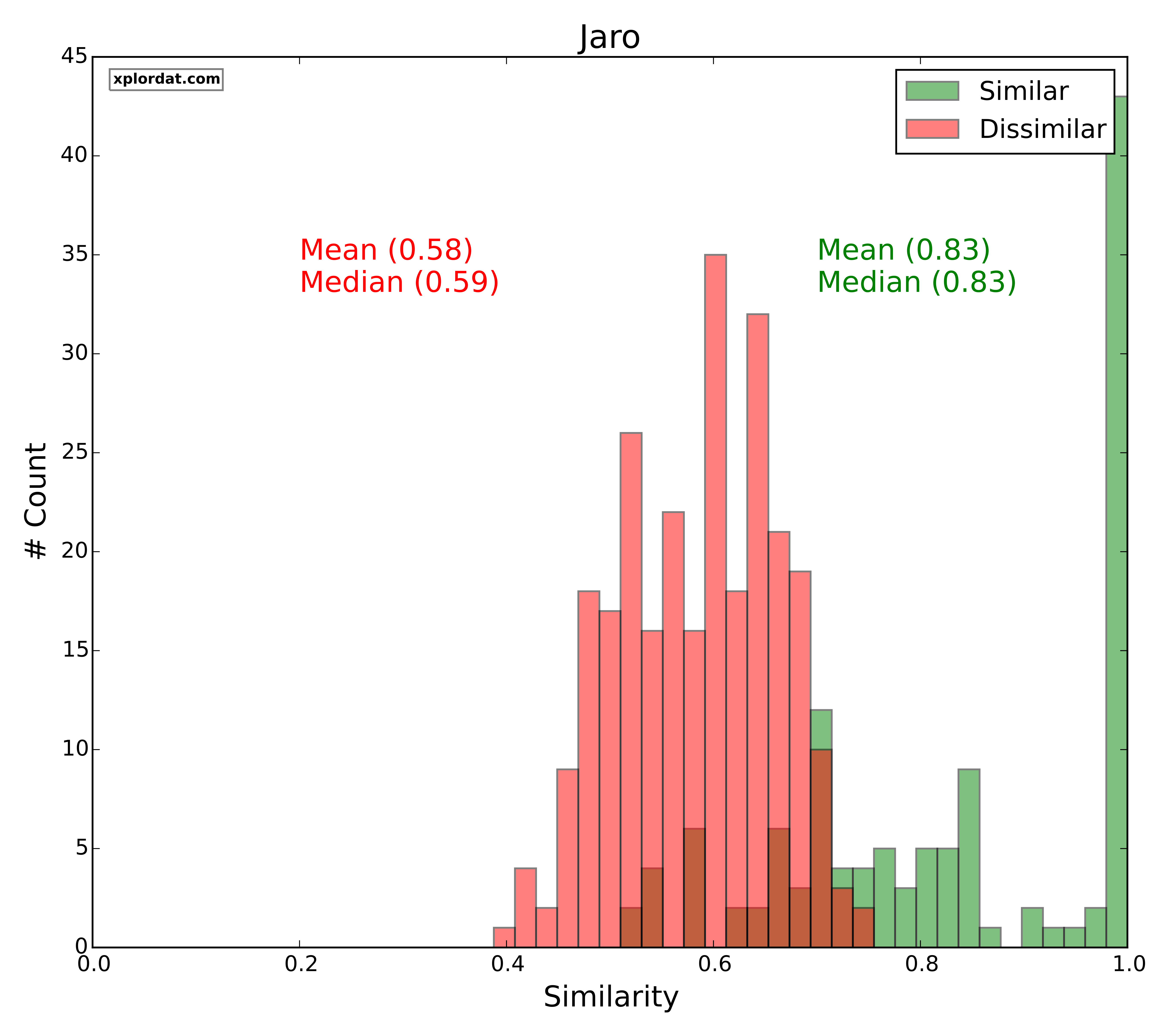
• Jaro > 0.8 => Lexically Similar
• Difflib Ratio > 0.6 => Lexically Similar

We simply ‘eyed’ the  cut-off numbers from the plots. Ideally it would be good to have even larger training set and establish some probabilities on getting false positives & false negatives when those numbers are used. We are running out of room here for this post but the idea can be readily implemented.

Larger & better training sets can improve results, but I would not say will substitute human oversight. Sure, it is sad that we do not have the computer doing all the work for us, but let us not put ourselves down, as we have made so much progress in having whittled down the potentially similar quotes to just a handful from thousands. Plus, we have found a way of surfacing up lexically similar quotes that have been incorrectly attributed. This approach can be readily productionized with minimal human intervention that approves/disapproves a quote being the same as an another. That was after all our limited objective for this post.