
Data streams are ubiquitous now-a-days. IOT devices, ATM transactions, apps, sensors etc… pushing out a steady stream of data. Analyzing these streams of data as they arrive poses challenges – especially when the data streams are coupled. They would be coupled for example when a single underlying process is generating multiple streams of data. Coupled data streams can only be analyzed together, paying particular attention to the simultaneity in time (and other process specific concerns such as the spatial location emitting the stream) of events across those streams. If one of the data streams gets delayed for whatever reason – the whole processing framework grinds to a halt waiting for it to catch up, while the data from the other streams piles up.
Waiting until all the data is in to make sense of it – does not apply. All the data will never be in at any time. Stream processing techniques batch the flowing data into chunks by windows in time and analyze each chunk as a batch. As there are different types of time – event/log/process etc… the specific time quantity to use to batch the stream depends on the process that is generating the data and the objective of the analysis. So does the specific type of the time-window (fixed-width, overlapping etc…) to use and their width. Slowly evolving phenomena can live with larger time-windows, while highly dynamic systems will need thin enough time-windows to faithfully track the process variations in time. Each window of data may yield a few metrics on the process at a representative time for that window – say its mid point.
It is an Imperfect World
Data streams in real world are never perfect so the stream processing framework has to plan for dealing with them.
- Late, out-of-order arrivals, and no-shows. Some old measurements may get delayed on their way and arrive later than newer measurements. Some may get lost altogether. How long should a time-window be kept open is a question that has no strict correct answer. It depends on the mechanisms producing and transporting the data to the processing framework.
- Early and improving results. There should be no need to wait for a time-window to close before processing that batch of data – especially when we need to keep the time-window open for late arrivals. Computing early metrics, even while they are approximate may be useful for detecting and alerting on potential issues.
- Need for simultaneity. Most processes produce different data streams at different rates. For example, a chemical reactor may have temperature and pressure sensors at different locations, each generating a stream of data. Any analysis of the reactor health will need the temperature and pressure measurements for the same time and from all the locations. That is, one cannot use the temperature measurement at one time and a pressure measurement a few minutes later (or at a different location) to correctly assess the reactor’s health.
The purpose of this post is to illustrate the above on simulated data streams. As for the stream processing framework, we will use Apache Beam as it seems quite well designed to address real world data streams. Besides, Beam provides a portable API layer to build parallel data processing pipelines that can be executed on a variety of execution engines – called runners, including Google Cloud DataFlow for scale. We will stick with DirectRunner here that runs locally. We will use Apache Kafka to produce data streams, and consume them in the Beam pipeline. The implementation code can be obtained from github.
1. The Data Streams
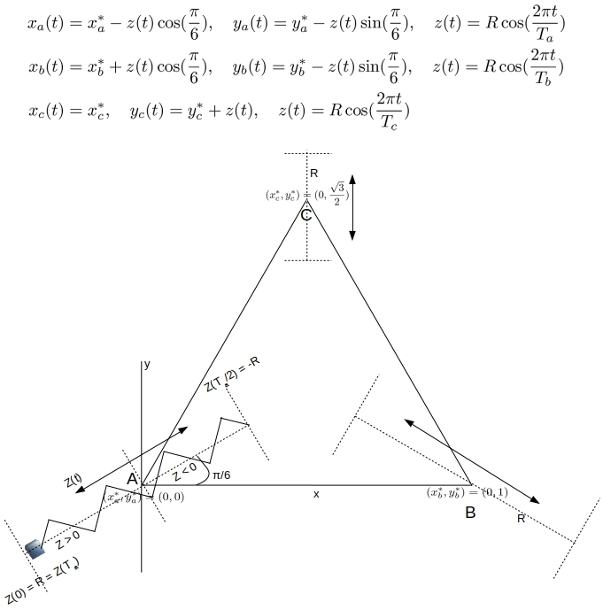
Consider three points that identify a well-defined triangle. Let an ideal mass-spring system be attached at each point and released at its extreme outer position when the experiment starts. As the points execute a simple harmonic motion around their rest states with different frequencies, their coordinate locations (x, y) generate a steady stream of data. Accurate estimates for metrics such as the perimeter and area of the triangle identified by these three points are of interest as this triangle deforms.The idealized triangle here is just a stand-in for say a triangular metallic flange holding up critical junctions, with data streams issuing out of the position monitors at each corner for example. Figure 1 below illustrates this and obtains the coordinate positions as explicit functions of time.
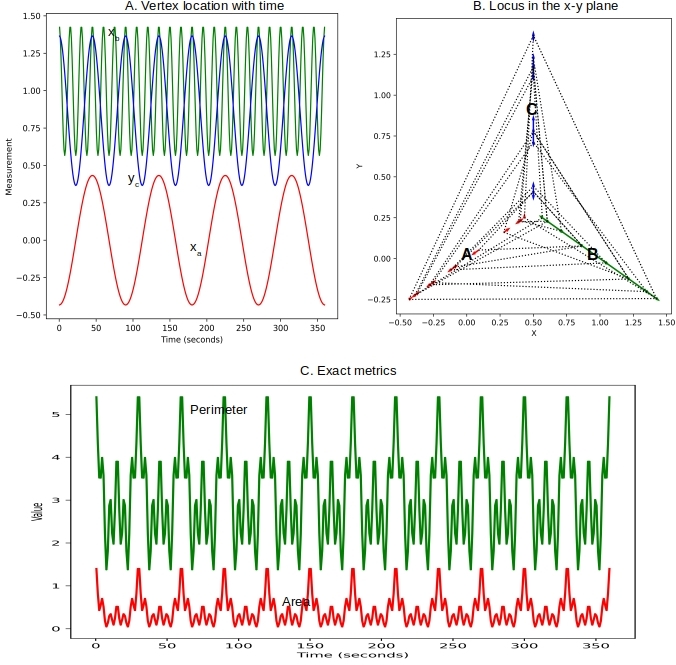
Given these equations, we can readily compute triangle metrics such as perimeter and area. Figure 2 below shows vertex A completing a full revolution in 90 seconds, where as B oscillates much faster taking only 15 seconds. As the vertices move in different ways, the area and perimeter of the triangle change in some chaotic fashion. But they do show a strict periodicity of 90 seconds – as Ta is a simple multiple of Tb and Tc .
2. The Data Streams
The (x, y) coordinates of the vertices are published to a Kafka topic – the source of the data stream. The actual measurement time is the create time of the event in the topic. But the events are randomly delayed so arrive into the topic in quite a different order as shown in Figure 3 below. Of course the arrival time is strictly later than the creation time for every measurement.
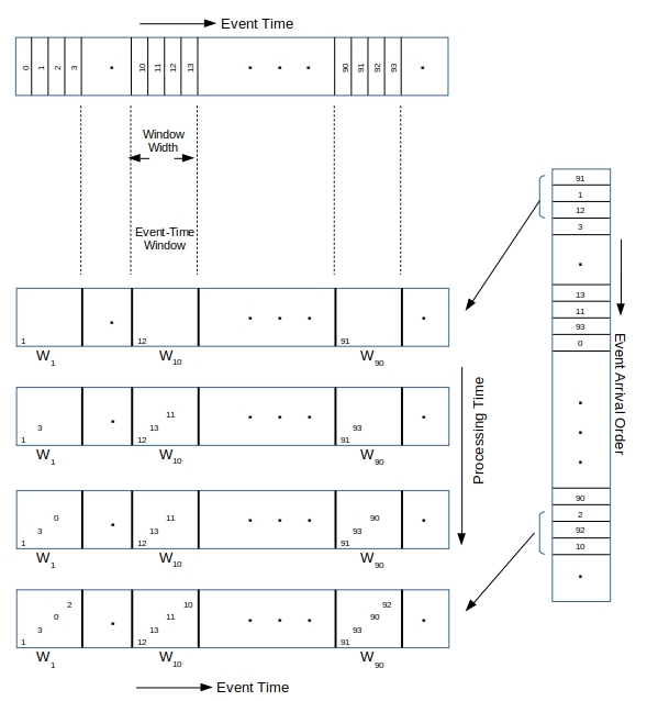
Figure 3 shows time-windows filling up with events as they arrive into the topic/stream. Given the simulated randomized delays, the first time-window continues to see events fall into it until the end. And the last time-window sees some events come in from the get go. Figure 4 below shows a event production order vs arrival order from one of the simulations.

In an ideal situation each time-window need only stay open for the duration of its width, from the moment the first event falls into that window. But given the out-of-order and late arrivals here, the time-windows need to stay open for much longer in order to avoid data loss.
3. Stream Processing
The objective of the stream processing is to compute the area and perimeter of the triangle as a function of time. This requires that a triangle be first identified in each time-window. A well-defined triangle requires the positions of all three vertices and at the same time. As the three monitors are not making synchronous measurements, we need to estimate the location of each vertex at a common instant – say the mid point of the time-window they fall in.
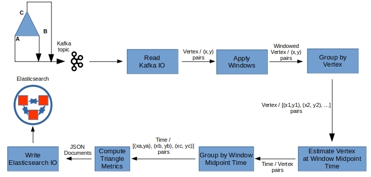
Figure 5 illustrates the machinations we put the data through to yield what we are after. Beam provides handy IO modules to talk to a variety of data sources and sinks. Here we read the events from a Kafka topic and eventually write out the metrics to Elasticsearch for analysis. Each step (except ‘Apply Windows’ which simply groups of data by event-time in windows) in the above takes a collection of elements as input and transforms them into an another collection of elements that feed to the next step.
3.1 Keys are the key to simultaneity and parallelism
Choosing (or building them if they do not exist in the data) the right keys to group the data is important for ensuring locality and simultaneity in time. Grouping by the vertex as the key first fixes the vertex for the next processing step, which computes & emits the estimated location of that vertex at some common time-instant (like the window mid-point) for all vertices. Grouping by this time-instant yields the three vertices at the same time-instant, for the next step that defines a triangle and compute its metrics for that time-instant.
In addition, the parallelism is switched from the number of vertices to the number of time-windows. Beam parallelism is builtin at the element level for each transform step. Our elements are key-value pairs. If for example we are monitoring data from say 10 triangular flanges, the first grouping can yield 30 concurrent executions. And, if we choose to estimate vertex locations at say 5 instants within each time-window, the second grouping yields a potential parallelism of five times the number of operating windows.
3.2 Interpolate for estimation
While this is not a Beam related concern, our specific problem here requires that we exercise some care in estimating the location of a vertex at window mid-point time. We may try a simple average, but this will only work when the location of the vertex does not change much over the duration of the time-window. It is better to interpolate as shown in Figure 6, by picking a few closest measurements from either side of the time instant for estimation.
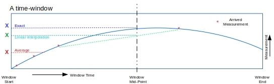
Further, a fast changing quantity will clearly require thin enough time-windows to capture its dynamics, and to approximate it with piecewise linears or (cubic splines perhaps) within the time-window.
3.3 Triggers
The time-windows continue to collect vertices until no more are left to arrive at which time the window will close. But there is no need to wait until that time as we can trigger the window pane to emit its contents every so often. When a window triggers, it publishes its contents so the subsequent steps get a new collection of elements to process and some triangle metrics get published out for analysis. Periodic triggering allows for early, if approximate metrics to be available right away.
The window can choose to accumulate its contents (as we do here) even after emitting them out periodically. This means a continual improvement in the metrics is possible as the estimation in Figure 6 gets closer to the exact value.
3.4 Pipeline code
The complete code to run these simulations here can be obtained from github. The pipeline set up for Beam is worth looking to confirm that it jives with what is depicted in Figures 5 and 6.
PCollection<KV<String, RawVertex>> vertices = pipeline
  .apply(KafkaIO.<String, GenericRecord>read() // Read from a kafka topic

  ...
// key is the vertex label: "A" , "B" or "C"
  .withKeyDeserializer(StringDeserializer.class)
// value is an Avro object
  .withValueDeserializer(ConfluentSchemaRegistryDeserializerProvider.of(schema_registry,topic+"-value")
  .withCreateTime(Duration.ZERO) // event createtime is used by Beam windows & watermark
  .apply(ParDo.of(new EmitRawVertex())); // PCollection<KV<String, RawVertex>>

PCollection<KV<String, RawVertex>> windowedVertices = vertices
// 1 second windows
  .apply(Window.<KV<String, RawVertex>>into(FixedWindows.of(Duration.standardSeconds(1)))
// keep the window open for a while to let in late arrivals
  .withAllowedLateness(Duration.standardSeconds(2*runTime), Window.ClosingBehavior.FIRE_ALWAYS)
// trigger after every time 15 new vertices come into a window
  .triggering(Repeatedly.forever(AfterPane.elementCountAtLeast(15)))
// Keep the earlier arrivals for improved estimations
  .accumulatingFiredPanes()) ; // PCollection<KV<String, RawVertex>>

windowedVertices
  .apply(GroupByKey.<String, RawVertex>create()) // PCollection<KV<String, <Iterable<RawVertex>>>
// Emit the vertex estimated (averaged or interpolated) at mid-point.
// Key is switched from vertex label to time
  .apply(ParDo.of(new EmitEstimatedVertex(vertex_estimation_strategy))) // PCollection<KV<Long, EstimatedVertex>>.
  .apply(GroupByKey.<Long, EstimatedVertex>create()) // PCollection<KV<Long, <Iterable<EstimatedVertex>>>
// Define a triangle and compute metrics
  .apply(ParDo.of(new EmitTriangle())) // PCollection<Triangle>>
  .apply(ParDo.of(new EmitJsonTriangle())) // PCollection<String>
  .apply(ElasticsearchIO.write() // write to Elasticsearch
    .withConnectionConfiguration(ElasticsearchIO.ConnectionConfiguration
      .create(esHosts, props.getProperty("es_triangle_index"))
      .withApiKey(props.getProperty("es_api_key"))

      ...

      )) ;
4. Results
Results are obtained for two different sets of periodicities for the vertices, and each time employing the two different ways (average or interpolate) of estimation. In the second set the vertices move three times faster relative to the first set – a case chosen to highlight the impact of interpolation strategy. So four runs in all, each running for 360 seconds, with Beam using 1-second fixed time-windows
- Ta=90, Tb=15, Tc=45. Estimate mid-point vertex by: Linear interpolation
- Ta=90, Tb=15, Tc=45. Estimate mid-point vertex by: Simple average
- Ta=30, Tb=5, Tc=15. Estimate mid-point vertex by: Linear interpolation
- Ta=30, Tb=5, Tc=15. Estimate mid-point vertex by: Simple average
Figure 7 shows the perimeter as a function of time for the base case – run 1.This basically validates the whole approach employed here for processing the three coupled streams to compute global metrics.

It is difficult to see in the figure above because of the scale, but both the first & final computed perimeter values in all the time-windows are in quite close agreement with the exact value. Let us look at this more closely. Figure 8 shows the ratio of computed to exact area with time in all four cases. Ideally we would want that to be 1.0.
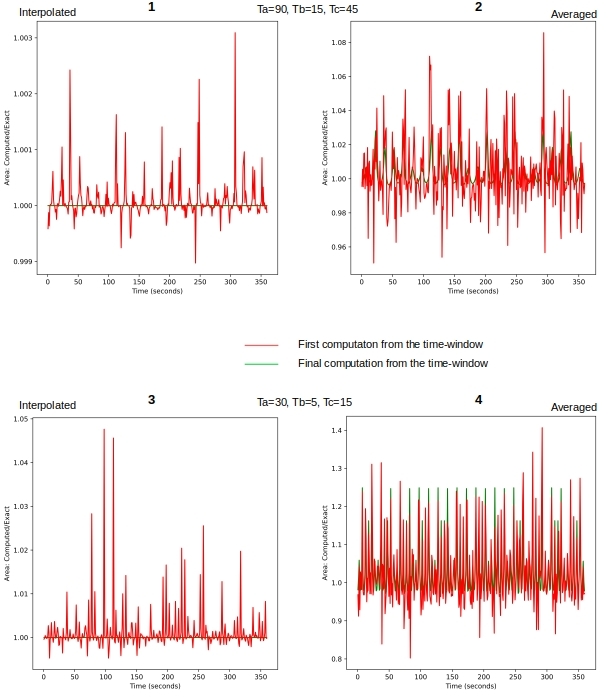
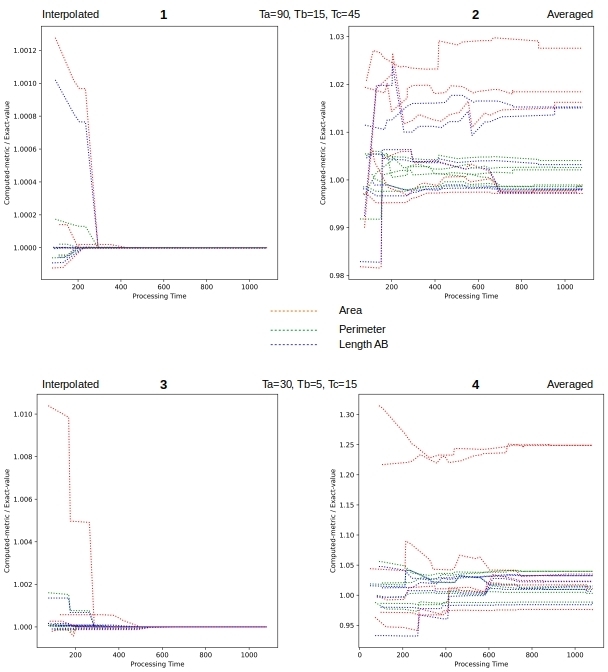
Figure 9 looks at the evolution of computed metrics from a given time-window. Somewhat similar to Figure 8 but includes all (i.e. not just the first & final) the values emitted for ametric over the life-time of the time-window. Once again we would hope to see improvement as we are accumulating the vertices. And we, do in case of interpolation and not so much when averaging.
5. Conclusions
Coupled data streams need to be analyzed together paying particular attention to simultaneity in event-time and other process specific variables controlling the data streams. With the help of a test problem with known exact solutions, we have shown that the pipeline processing with Beam can accurately obtain them.
Apache Beam provides the means to handle many of the challenges associated with processing coupled data streams – whether it is switching the keys as needed to suit the processing, allowing for late arrivals, and enabling early metrics etc… Plus the builtin parallelism at the element level and the exportability of the pipeline to execute on different runners makes Beam quite appealing for large scale stream processing.