BERT yields the best F1 scores on three different repositories representing binary, multi-class, and multi-label/class situations. BoW with tf-idf weighted one-hot word vectors using SVM for classification is not a bad alternative to going full bore with BERT however, as it is cheap.
Robots are reading, chatbots are chatting, and some are even writing essays apparently. There is a lot of buzz and excitement now-a-days in the NLP world. And for good reason too. Computers are learning to work with text and speech the way people do. Hal from 2001 may be finally here, a few years late as it may be. Joking aside, one of the core skills these bots are mastering is to classify text/speech on the fly so they can process further.
But the techniques for classifying a given set of vectors have not changed all that much over the years. Support Vector Machines (SVM) by Cortes and Vapnik in 1995 was perhaps the last significant advance. Clearly the buzz is coming from the upstream – where text is being converted to vectors. Better quality input vectors lead to better classification accuracy – by the same classification algorithm. If your document vectors are more faithfully embedding and reflecting the meaning of the documents – good for you! You will get more mileage out of your old classifiers. But who is cooking up all these good vectors upstream? Not Professor Septima Vector, for sure!
It turns out to be BERT and his friends ELMO and the like. In the earlier post BoW to BERT we have seen how the word vectors have evolved to adapt to the context they are operating in. We looked at similarity or lack thereof between two vectors of the same word, but in different contexts.
The purpose of this post is to see what difference all that agility of word vectors, makes for a practical downstream task – classification of documents. Here is a quick outline.
- Take three different document repositories. The movie reviews from Stanford (for binary sentiment classification), the 20-news corpus via scikit-learn (for multi-class classification) and the reuters corpus via NLTK (for multi-class & multi-label classification). Repeat 2 thru 4 for each of these repositories.
- Build BoW document vectors using 1-hot & fastText word vectors. Classify with Logistic Regression & SVM.
- Fine-tune BERT for a few epochs (5 here) while classifying on the vector shooting out of the top layer’s classification token [CLS]
- Compare the (weighted) F1 scores obtained in 2 and 3.
Logistic regression and SVM are implemented with scikit-learn. BERT is implemented as a Tensorflow 2.0 layer using the transformers module from huggingface. Let us get with it. We will go over some code snippets here but the complete code can be obtained from github.
1. Document vectors for classification
Bow is an approach to build a document vector out of the words (their numerical vectors to be specific, 1-hot, fastText etc…) in the document. We have gone over this in the previous post. Here is the equation we had.
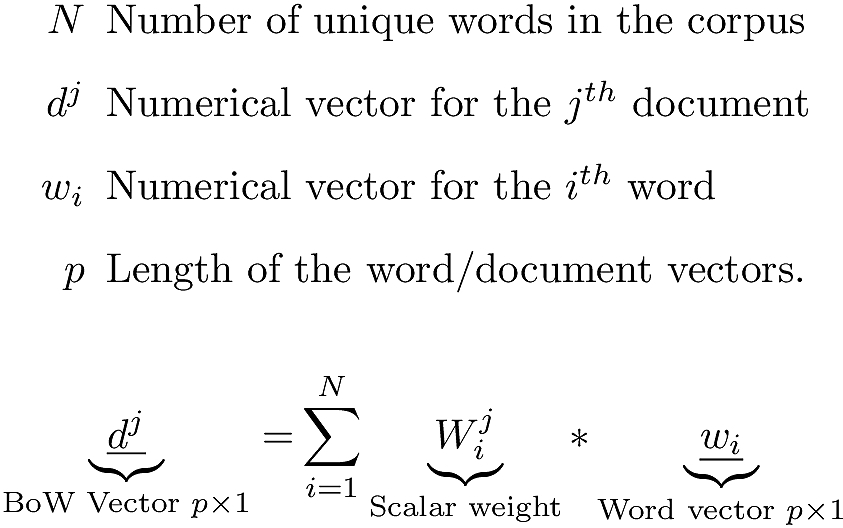
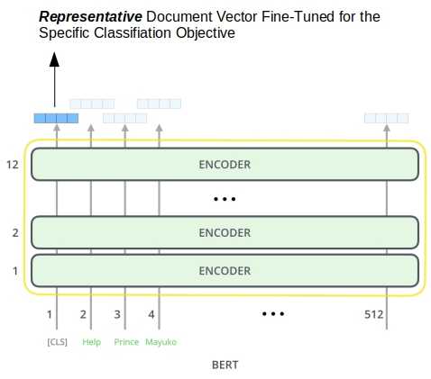
BERT can be used to generate word vectors and Equation 1 above can be used to obtain a document vector. But when classification is the downstream purpose, BERT does not need a document vector to be built from word vectors. The vector shooting out of the top layer’s ‘[CLS]’ token serves as a representative document vector fine-tuned for the specific classification objective. Here is a schematic (from Jay Alammar) of the smaller BERT model employing 12 layers, 110 million parameters, a maximum of 510 sequence of words. The word embeddings, and the CLS token vector used classification purposes are 768 long here.
Transfer learning and Fine tuning with BERT
The published word vectors such as those from fastText are trained on vast amounts of text. We can use them in our documents. That is, these word vectors are transferable. But they will not have incorporated any specific knowledge from our documents. Neither will they have any idea what we would be using them for. That is, they are both static and task agnostic. We can build custom fastText word vectors for our document corpus. Custom vectors embed corpus specific knowledge but not transferable to a different corpus. And they are task agnostic as well.
Fine tuning generic, transferable word vectors for the specific document corpus and for the specific downstream objective in question is a feature of the latest crop of language models like BERT.
BERT can yield numerical vectors for any word in a sentence (no longer than 510 tokens of course) with no additional training. But when possible, it is advantageous to further train BERT a bit with our documents against our objective. The word (and the CLS token) vectors thus obtained would then have learnt some new tricks to do well for our tasks and with our documents. Note that we say when possible. Even the smaller BERT is a beast with 110 million parameters. For large document repositories, it would be quite expensive to fine-tune BERT. Luckily for us, our repos are not so huge.
2. Document and label vectors
The documents are cleaned up with a simple regex like the one below. Joining these tokens back up with a space character would yield our cleaned document.
def tokenize (text): # no punctuation & starts with a letter & between 2-15 characters in length
    tokens = [word.strip(string.punctuation) for word in RegexpTokenizer(r'\b[a-zA-Z][a-zA-Z0-9]{2,14}\b').tokenize(text)]
    return  [f.lower() for f in tokens if f]
The number of words in the documents is important to us, because BERT is limited to 510 words per document. Actually 512, but the other two are taken up by the special start ([CLS]) and end ([SEP]) tokens. Figure 2 shows the vitals of these repos including the distribution of the number of words. Note that vast bulk of the documents fall under 510 words, meaning BERT should be happy. But BERT is resource intensive and on my computer it could only work with about 175 words per document (with 32 as the batch size), before running into OOM issues.
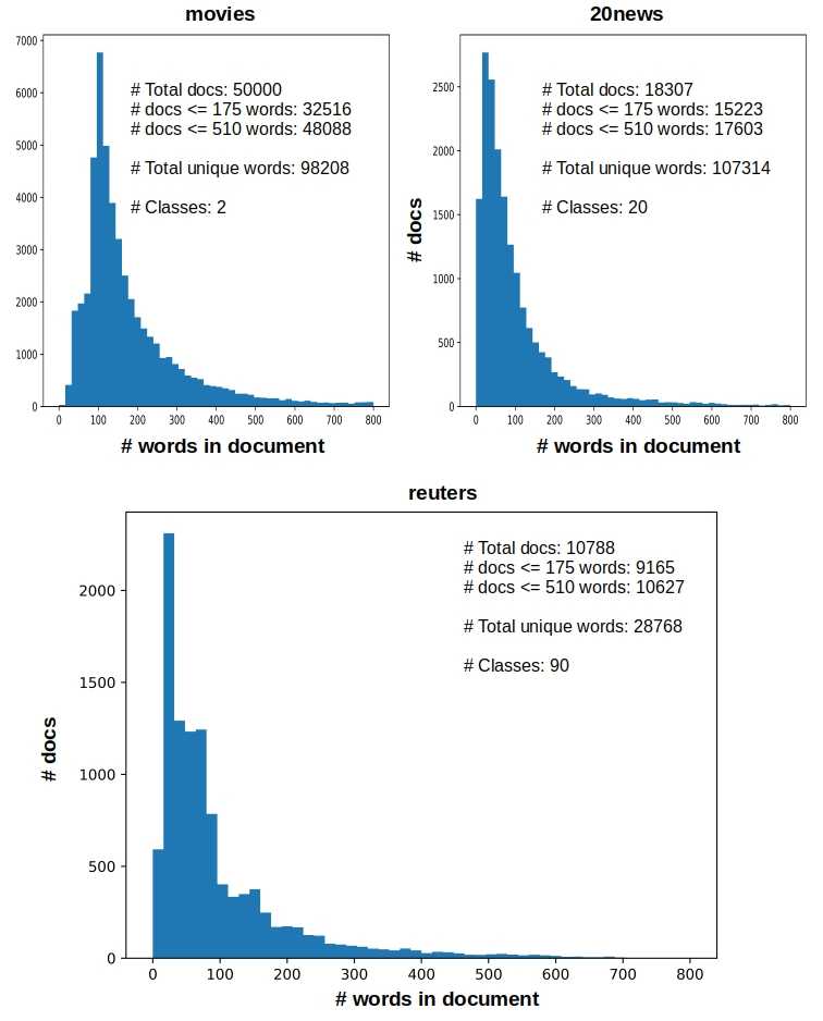
Figure 3 shows the distribution of class labels for the repos. It is quite important to know. Care has to be taken in interpreting the performance of a classifier on skewed data sets.
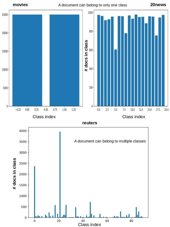
In all cases, the label vector for document is as long as the number of classes. It will have 1 at indices corresponding to the classes that it belongs to, and 0 elsewhere. So a label vector for a document in the reuters repo will be 90-long with as many values of 1 as the number of classes it belongs to. The label vectors in the other two repos are one-hot as a their documents can only belong to one class.
3. Classifying with Bow
For logistic regression and SVM we build Bow vectors as per Equation 1. Tf-idf weights are used for W^j_i. One-hot and fastText word vectors are tried for w_i. For fastText we use the 300-dim vectors, i.e. p = 300 in Equation 1. Here is a snippet of code to build tf-idf vectors with one-hot word vectors.
X = docs['train'] + docs['test'] # All docs
X=np.array([np.array(xi) for xi in X]) # rows: Docs. columns: words
vectorizer = TfidfVectorizer(analyzer=lambda x: x, min_df=1).fit(X)
word_index = vectorizer.vocabulary_ # Vocabulary has all words
train_x = vectorizer.transform(np.array([np.array(xi) for xi in docs['train']])) # sparse tf-idf vectors using 1-hot word vectors
test_x = vectorizer.transform(np.array([np.array(xi) for xi in docs['test']])) # sparse tf-idf vectors using 1-hot word vectors
When using fastText word vectors for w_i we get the embedding matrix W (each row represents a word vector of length p) from the published word vectors and multiply it with the above tf-idf sparse matrix.

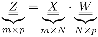
train_x = sparseMultiply (train_x, embedding_matrix)

def sparseMultiply (sparseX, embedding_matrix):
    denseZ = []
    for row in sparseX:
        newRow = np.zeros(wordVectorLength)
        for nonzeroLocation, value in list(zip(row.indices, row.data)):
            newRow = newRow + value * embedding_matrix[nonzeroLocation]
        denseZ.append(newRow)
    denseZ = np.array([np.array(xi) for xi in denseZ])
    return denseZ
Using these vectors to classify with logistic regression or SVM is straightforward with scikit-learn. The reuters corpus is multi-class & multi-label so we need to wrap the models in a OneVsRestClassifier. The multi-label confusion marix from this is summed up here to get a weighted confusion matrix.
if (clf == 'svm'):
    model = LinearSVC(tol=1.0e-6,max_iter=20000)
elif (clf == 'lr'):
    model = LogisticRegression(tol=1.0e-6,max_iter=20000)
if (docrepo == 'reuters'):
    classifier = OneVsRestClassifier(model)
    classifier.fit(train_x, y['train'])
    predicted = classifier.predict(test_x)
    mcm = multilabel_confusion_matrix(y['test'], predicted)
    tcm = np.sum(mcm,axis=0) # weighted confusion matrix
else:
    train_y = [np.argmax(label) for label in y['train']]
    test_y = [np.argmax(label) for label in y['test']]
    model.fit(train_x, train_y)
    predicted = model.predict(test_x)
    cm = confusion_matrix(test_y, predicted)
4. Classifying with BERT
As we said earlier BERT does not need Bow vectors for classification. It builds them as part of fine-tuning for the specific classification objective. BERT has its own tokenizer, and vocabulary. We use its tokenizer and prepare the documents in a way that BERT expects.
The snippet of code below takes a list of documents, tokenizes them generates the ids, masks, and segments used by BERT as input. Each document yields 3 lists, each of which is as long as max_seq_length – the same for all documents. Documents longer than max_seq_length tokens are truncated. Documents shorter than max_seq_length tokens are post-padded with 0’s until they have max_seq_length tokens. max_seq_length itself is limited to a maximum of 510.
import tensorflow as tf # 2.0
from transformers import *

tokenizer = BertTokenizer.from_pretrained('bert-base-uncased') #  BertTokenizer from the transformers module
def prepareBertInput(tokenizer, docs):
    all_ids, all_masks, all_segments= [], [], []
    for doc in tqdm(docs, desc="Converting docs to features"):
        tokens = tokenizer.tokenize(doc)
        if len(tokens) > max_seq_length:
            tokens = tokens[0 : max_seq_length]
        tokens = ['[CLS]'] + tokens + ['[SEP]']
        ids = tokenizer.convert_tokens_to_ids(tokens)
        masks = [1] * len(ids)
        # Zero-pad up to the sequence length.
        while len(ids) < max_seq_length:
            ids.append(0)
            masks.append(0)
        segments = [0] * max_seq_length
        all_ids.append(ids)
        all_masks.append(masks)
        all_segments.append(segments)
    encoded = [all_ids, all_masks, all_segments]
    return encoded
Figure 4 below runs the above for a couple of sentences. Each list of actual tokens for a document is prepended with a special token ‘[CLS]’ and appended with ‘[SEP]’. The ids are simply integer mappings from BERT vocabulary. A mask of 0 indicates a padded token that is to be ignored. The segments are simply zero vectors for our single document classification problems.

The transformers module can load a pre-trained BERT model as a TensorFlow 2.0 tf.keras.Model sub-class object. This makes it seamless to integrate with other Keras layers in building a custom model around BERT. Before we define the full model though we should accommodate for the multi-label situation for the reuters repo.
if (docrepo == 'reuters'):
  multiLabel = True
  tfMetric = tf.keras.metrics.BinaryAccuracy()
  tfLoss = tf.losses.BinaryCrossentropy()
  activation = 'sigmoid'
  allMetrics = [tfMetric, tf.metrics.FalsePositives(), tf.metrics.FalseNegatives(), tf.metrics.TrueNegatives(), tf.metrics.TruePositives(), tf.metrics.Precision(), tf.metrics.Recall()]
else:
  multiLabel = False
  tfMetric = tf.keras.metrics.CategoricalAccuracy()
  tfLoss = tf.losses.CategoricalCrossentropy()
  activation = 'softmax'
allMetrics = [tfMetric]- In the multi-label case, the presence of a label should not impact the presence/absence of another. So the final dense layer needs a sigmoid activation. If the predicted score for any label is greater than 0.5, then the document is assigned that label.
- Softmax activation is suitable for the single-label case. It forces the sum of all the probabilities to be 1 creating a dependence among them. This is fine for single-label case as the labels are mutually exclusive and we pick the label with the highest predicted probability as the predicted label.
- The binary metric looks at the predicted probability for each label and if it is greater than 0.5 it tallies a hit (say 1) or a miss (say 0) otherwise. So a single predicted vector yields multiple 1’s and 0’s contributing to the overall predictive capability across all documents and labels.
- The categorical metric on the other hand looks for the label with the maximum predicted probability and yields a single 1 (for a hit) or a single 0 (for a miss). This is appropriate for the single-label case.
- The other TF supplied metrics such as tf.metrics.FalsePositives() employ a default threshold of 0.5 for the probability and so are suitable to be tracked for the multi-label case.
With that discussion of the way, we are ready to define the model.
def getModel():
    in_id = tf.keras.layers.Input(shape=(max_seq_length,), dtype='int32', name="bert_input_ids")
    in_mask = tf.keras.layers.Input(shape=(max_seq_length,), dtype='int32', name="bert_input_masks")
    in_segment = tf.keras.layers.Input(shape=(max_seq_length,), dtype='int32', name="bert_segment_ids")
    inputs = [in_id, in_mask, in_segment]
    top_layer_vectors, top_cls_token_vector = TFBertModel.from_pretrained(BERT_PATH, from_pt=from_pt)(inputs)
    predictions = tf.keras.layers.Dense(len(labelNames), activation=activation,use_bias=False)(top_cls_token_vector)
    model = tf.keras.Model(inputs=inputs, outputs=predictions)
    model.compile(optimizer=tf.optimizers.Adam(learning_rate=2e-5, epsilon=1e-08, clipnorm=1.0), loss=tfLoss, metrics=allMetrics)
    return model
Line #6 in the above snippet loads the ‘uncased_L-12_H-768_A-12’ model as a layer taking the prepared inputs. It employs 12 layers (transformer blocks shown in Figure 1), 12 attention heads and 110 million parameters. Each token has a 768-long numerical vector representation in each layer. The ‘top_cls_token_vector’ is the 768 long vector shooting out of the top layer’s ‘[CLS]’ token.
Here is the schematic of the above Keras model for the binary classification of movies, employing a maximum of 175 words for any document. The image shows 177 because of the two special tokens we mentioned earlier.

5. Results
Just so all runs use the exact same documents, and train/test splits, we prepare them in advance. A shell script runs the various combinations of repositories and classifiers, saving the results for analysis. With the BoW approach there are 36 combinations.
- 3 repos (movies, 20news, reuters)
- 2 classifiers (Logistic regression, SVM)
- 2 types of word vectors (One-hot, fastText), and
- 3 different values for the maximum number of words considered per document (175, 510, ALL). The reason to consider these is to be able to compare head-2-head against BERT that can only handle a maximum of 510 tokens, and more like 175 on my desktop due to OOM issues.
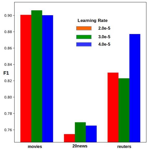
With BERT there are only 3 runs – one for each of the repos. While BERT is limited to 510 tokens anyway, practical limitations on my desktop would only allow 175 at the batch size of 32. The base ‘uncased_L-12_H-768_A-12’ model is loaded from s3 and fine tuned for 5 epochs. There is some impact with learning rate that is explored separately.
history = model.fit(encoded['train'], y['train'], verbose=2, shuffle=True, epochs=5, batch_size=32)
evalInfo = model.evaluate(encoded['test'], y['test'], verbose=2)
Figure 6 below is what we are after and it took the whole blog to get to it. The weighted F1 score across all labels is what we compare as the support across labels is quite different especially in the case of reuters as we saw in Figure 3. Here are some easy conclusions.
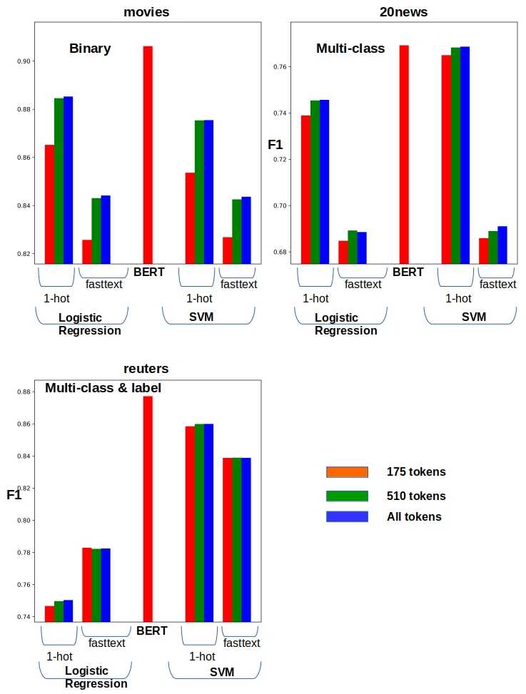
- BERT yields the best F1 scores in all cases.
- Using more tokens, Logistic regression and SVM slightly improve their scores. But BERT with 175 tokens is still the leader. Most of the documents have fewer than 175 words anyway as we have seen in Figure 2.
- One-hot word vectors are perhaps to be preferred over fastText. In fact, slapping a BoW on one-hot word vectors and using SVM as the classifier yields pretty good F1 scores.
- Perhaps an easy, cheap shot but the outperformance of BERT is also accompanied by a much, much higher utilization of resources compared to BoW.
We mentioned in passing earlier that the learning rate during fine tuning has some impact on the obtained results with BERT. Figure 7 below illustrates it. Optimizing for hyper parameters when using BERT is a computational challenge as well.
6. Conclusions
When classification is the objective, BoW with tf-idf weighted one-hot word vectors and traditional approaches such as SVM should be the first thing to try. It will establish a baseline we can aim to beat with newer approaches such as BERT. BERT yields high quality results at some expense. But faster and lighter versions of BERT are being explored constantly, and compute is getting cheaper as well with cloud options. Plus BERT embeddings are not limited to producing a sentence vector for classification and the one-hot and fastText embeddings have nothing on BERT for those other use cases.
With that we conclude this post. We will look at using BoW with BERT for clustering in an upcoming post.


Hello Ashok,
Thanks for great article!
Could you provide link to full code?
Hi Evgeny,
Yeah, I need to clean it up and put it on github. Hope to get to it in the next few days.
Hi Evgeny,
Finally got around to it. Please find the complete code at https://github.com/ashokc/BoW-vs-BERT-Classification
Nice example!
What is the `metrics` module in the statement `from metrics import Metrics.` I get an error there I can’t fine it with a web search.
Thanks for pointing this out Justin. It is just a package/file I wrote to compute the various metrics. Forgot to check it in to GitHub at the time. It is in there now
I get an error with the statement `from metrics import Metrics`. Where can I find this module?
Just found your comment buried in the mail, Justin. My apologies!
You are right. I had forgotten to check that script in. It is just a class to compute the various classification metrics