
Logistic Regression has traditionally been used as a linear classifier, i.e. when the classes can be separated in the feature space by linear boundaries. That can be remedied however if we happen to have a better idea as to the shape of the decision boundary…
Logistic regression is known and used as a linear classifier. It is used to come up with a hyperplane in feature space to separate observations that belong to a class from all the other observations that do not belong to that class. The decision boundary is thus linear. Robust and efficient implementations are readily available (e.g. scikit-learn) to use logistic regression as a linear classifier.
While logistic regression makes core assumptions about the observations such as IID (each observation is independent of the others and they all have an identical probability distribution), the use of a linear decision boundary is not one of them. The linear decision boundary is used for reasons of simplicity following the Zen mantra – when in doubt simplify. In those cases where we suspect the decision boundary to be nonlinear, it may make sense to formulate logistic regression with a nonlinear model and evaluate how much better we can do. That is what this post is about. Here is the outline. We go through some code snippets here but the full code for reproducing the results can be downloaded from github.
- Briefly review the formulation of the likelihood function and its maximization. To keep the algebra at bay we stick to 2 classes, in a 2-d feature space. A point [x, y] in the feature space can belong to only one of the classes, and the function f (x,y; c) = 0 defines the decision boundary as shown in Figure 1 below.

- Consider a decision boundary that can be expressed as a polynomial in feature variables but linear in the weights/coefficients. This case lends itself to be modeled within the (linear) framework using the API from scikit-learn.
- Consider a generic nonlinear decision boundary that cannot be expressed as a polynomial. Here we are on our own to find the model parameters that maximize the likelihood function. There is excellent API in the scipy.optimize module that helps us out here.
1. Logistic Regression
Logistic regression is an exercise in predicting (regressing to – one can say) discrete outcomes from a continuous and/or categorical set of observations. Each observation is independent and the probability p that an observation belongs to the class is some ( & same!) function of the features describing that observation. Consider a set of n observations [x_i, y_i; Z_i] where x_i, y_i are the feature values for the ith observation. Z_i equals 1 if the ith observation belongs to the class, and equals 0 otherwise. The likelihood of having obtained n such observations is simply the product of the probability p(x_i, y_i) of obtaining each one of them separately.
(1) ![\begin{align*}L = & \prod_{i=1}^{n} p_i^{Z_i} \, (1-p_i)^{(1-Z_i)} \\ \log{L} = & \sum_{i=1}^{n} \left[ Z_i \log{\frac{p_i}{1-p_i}} + \log{(1-p_i)} \right]\end{align*}](https://xplordat.com/wp-content/ql-cache/quicklatex.com-5cc2a405bb6443cab0375bd53dbb2d81_l3.png "Rendered by QuickLaTeX.com")
The ratio p/(1-p) (known as the odds ratio) would be unity along the decision boundary as p = 1-p = 0.5. If we define a function f(x,y; c) as:
(2) 
then f(x,y; c) =0 would be the decision boundary. c are the m parameters in the function f. And log-likelihood in terms of f would be:
(3) ![\begin{equation*}\log{L} = \sum_{i=1}^{n} \left[ Z_i f_i - \log{(1 + e^{f_i})} \right]\end{equation*}](https://xplordat.com/wp-content/ql-cache/quicklatex.com-a3e3a569457942d8694f2c558c79e837_l3.png "Rendered by QuickLaTeX.com")
All that is left to be done now is to find a set of values for the parameters c that maximize log(L) in Equation 3. We can either apply an optimization technique or solve the coupled set of m nonlinear equations d log(L)/dc = 0 for c.
(4) ![\begin{align*}\frac{d \log{L}}{dc_j} = & \sum_{i=1}^{n} \left[ Z_i - \frac{1}{1 + e^{-f_i}} \right] \left( \frac{df}{dc_j} \right)_i \quad \quad \forall j = 1, 2, ... m \\ \frac{d \log{L}}{dc} = & \underbrace{ \begin{bmatrix} \frac{df_1}{dc_0} & \frac{df_2}{dc_0} & \hdots & \frac{df_N}{dc_0} \\ \frac{df_1}{dc_1} & \frac{df_2}{dc_1} & \hdots & \frac{df_N}{dc_1} \\ \cdots \\ \frac{df_1}{dc_m} & \frac{df_M}{dc_m} & \hdots & \frac{df_n}{dC_m}\end{bmatrix}}_{m \times n} \cdot \underbrace{ \begin{bmatrix} Z_1 - \frac{1}{1+e^{-f_1}} \\ Z_2 - \frac{1}{1+e^{-f_2}} \\ \cdots \\ Z_N - \frac{1}{1+e^{-f_n}} \end{bmatrix}}_{n \times 1} = 0 \end{align*}](https://xplordat.com/wp-content/ql-cache/quicklatex.com-900ea524412c3055b12f1a76d0e52ff1_l3.png "Rendered by QuickLaTeX.com")
Either way, having c in hand completes the definition of f and allows us find out the class of any point in the feature space. That is logistic regression in a nut shell.
2. The function f(x,y; c)
Would any function for f work in Equation 2? Most certainly not. As p goes from 0 to 1, log(p/(1-p)) goes from -inf to +inf. So we need f to be unbounded as well in both directions. The possibilities for f are endless so long as we make sure that f has a range from -inf to +inf.
2.1 A linear form for f(x,y; c)
Choosing a linear form such as
(5) 
will work for sure and that leads to traditional logistic regression as available for use in scikit-learn and the reason logistic regression is known as a linear classifier.
2.2 A higher-order polynomial for f(x,y; c)
An easy extension Equation 5 would be to use a higher degree polynomial. A 2nd order one would simply be:
(6) 
Note that the above formulation is identical to the linear case, if we treat x^2, xy, and y^2 as three additional independent features of the problem. The impetus for doing so would be that we can then directly apply the API from scikit-learn to get an estimate for c. We see however in the results section that the c obtained this way is not as good as directly solving Equation 4 for c. It is a bit of a mystery as to why. But in any case solving Equation 4 is easy enough with modules from scipy. The derivatives we need for Equation 4 fall out simply as
![\[\frac{df}{dc_0} = 1 \quad \frac{df}{dc_1} = x \quad \frac{df}{dc_2} = y\ \quad \frac{df}{dc_3} = x^2 \quad \frac{df}{dc_4} = xy \quad \frac{df}{dc_5} = y^2 \]](https://xplordat.com/wp-content/ql-cache/quicklatex.com-100fe83efb01e4434442a6e2d86e2f01_l3.png "Rendered by QuickLaTeX.com")
2.3 Other generic forms for f(x,y; C)
A periodic form like f(x,y; c) = sin(c_0x + c_2y) = 0 will not work as its range is limited. But the following will.
(7) 
We can again evaluate the derivatives and solve for the roots of Equation 4 but sometimes it is simpler to just directly maximize log(L) in Equation 3, and that is what we will do in the simulations to follow.
3. Simulations
We generate equal number of points in the x, y feature space that belong to a class (Z = 0 when f(x,y; c) > small_value) and those that do not belong (Z = 1 when f(x, y; c) < small_value) as we know the explicit functional form of f(x,y; c).
nPoints = 1000
def generateData():
    x = (xmax - xmin) * np.random.random_sample(nPoints*25) + xmin
    y = (ymax - ymin) * np.random.random_sample(nPoints*25) + ymin
    allData = np.stack((x, y),axis=-1)
    fvals = getF (true_c, allData) # True decision boundary
    data, Z = [], []
    zeroCount, oneCount = 0, 0
    for i,f in enumerate(fvals):
        if ( (zeroCount < nPoints) and (f > 1.0e-2) ):
            Z.append(0.0)
            data.append(allData[i])
            zeroCount = zeroCount + 1
        if ( (oneCount < nPoints) and (f < -1.0e-2) ):
            Z.append(1.0)
            data.append(allData[i])
            oneCount = oneCount + 1
        if (zeroCount == nPoints) and (oneCount == nPoints):
            break;
    data=np.array([np.array(xi) for xi in data])
    Z = np.array(Z)
    return data, Z
The data is split 80/20 for train vs test. We use the API from scikit-learn for the linear case that we want to compare with.
sss = StratifiedShuffleSplit(n_splits=1, test_size=0.2, random_state=1).split(data, Z)
train_indices, test_indices = next(sss)
data_train = data[train_indices]
Z_train = Z[train_indices]

lr = LogisticRegression(max_iter=10000, verbose=0, tol=1.0e-8, solver='lbfgs' )
lr.fit(data_train, labels_train)
linear_predicted_labels = lr.predict(data[test_indices])
linear_c = np.array([lr.intercept_[0], lr.coef_[0][0], lr.coef_[0][1]]) / lr.intercept_[0] # scaled so we can compare the coefficient values across different approaches
We use the scipy.optimize module when choosing to solve the Equations in 4 for c or for maximizing the likelihood in Equation 3. LL and dLLbydc in the code snippet below are simply implementing Equations 3 and 4 respectively. The scipy routines are for minimization so we negate the sign in each case as we want to maximize the likelihood.
from scipy import optimize
def getLLforMin(c):
    f = getF(c, data_train)
    LL = np.dot(Z_train.T, f) - np.sum (np.log(1.0 + np.exp(f)))
    return -LL
def getdLLbydcforMin(c):
    f = getF(c, data_train)
    dfbydc = getFprime(c, data_train)
    dLLbydc = np.dot(dfbydc.T, Z_train - 1.0/(1+np.exp(-f)))
    return -dLLbydc
Finally we solve for c starting with a small initial guess close to 0.
cguess = true_c * 1.0e-3
root_minimize = optimize.minimize(getLLforMin, cguess)
root_solve = optimize.fsolve(getdLLbydcforMin, cguess)
4. Results
We look at the polynomial and the other generic case separately.
4.1 f(x,y; c) = c_0 + c_1 x + c_2 y + c_3 x^2 + c_4 x y + c_5 y^2
We get an ellipse as the decision boundary for the following c values
![\[f(x,y; c) = 2.25 -3x -18y + 35x^2 - 64xy + 50y^2 = 0\]](https://xplordat.com/wp-content/ql-cache/quicklatex.com-3ead75bfb98bb9be05562a257b656832_l3.png "Rendered by QuickLaTeX.com")
We generate 1000 data points for each class based on the above function and apply logistic regression to that data to see what it predicts for the decision boundary.
pipenv run python ./polynomial.py 1000 2.25 -3.0 -18.0 35.0 -64.0 50.0Figure 2 below shows the data distribution and the decision boundaries obtained by the different approaches. The contour traced by green triangles separates the data perfectly, i.e. gets an F1 score of 1. It is obtained by solving Equation 4 for c. The red line is obtained by the traditional logistic regression approach – clearly a straight line. It tries to do the best it can given the nonlinearities and gets an F1 score of well 0.5… The contour traced by the blue triangles is interesting. It is obtained by applying traditional logistic regression on augmented feature space. That is “x^2”, “x*y”, and “y^2” are treated as three additional features thereby linearizing f for use with scikit-learn. It gets an F1 score of 0.89 which is not bad. But it is not entirely clear why it should be worse than solving dlog(LL)/dc = 0.

The actual values for the coefficients are shown in Table 1 below. c_0 is scaled to unity so we can compare. Clearly the coefficients obtained solving dlog(LL)/dc = 0 are closest to the actual values used in generating the data.
| Method | c_0 | c_1 | c_2 | c_3 | c_4 | c_5 | F1 |
| Actual values | 1 | -1.333 | -8 | 15.555 | -28.444 | 22.222 | |
| Solving dlog(LL)/dc = 0 | 1 | -1.305 | -7.919 | 15.143 | -27.661 | 21.756 | 1.0 |
| scikit-learn with augmented features | 1 | -3.281 | -7.076 | 9.999 | -13.301 | 13.983 | 0.889 |
| Default scikit-learn | 1 | 0.751 | -2.765 | 0.5 |
4.2 f(x,y; c) = c_0 + c_1 sin(c_2 x^2) + c_3 y = 0
Figure 3 shows the data distribution and the predicted boundaries upon running the simulation with
pipenv run python ./generic.py 1000 1.0 -1.0 1.0 -1.0The straight line from traditional logistic regression obtains an F1 score of 0.675 whereas the direct minimization of log(LL) gets a perfect score.
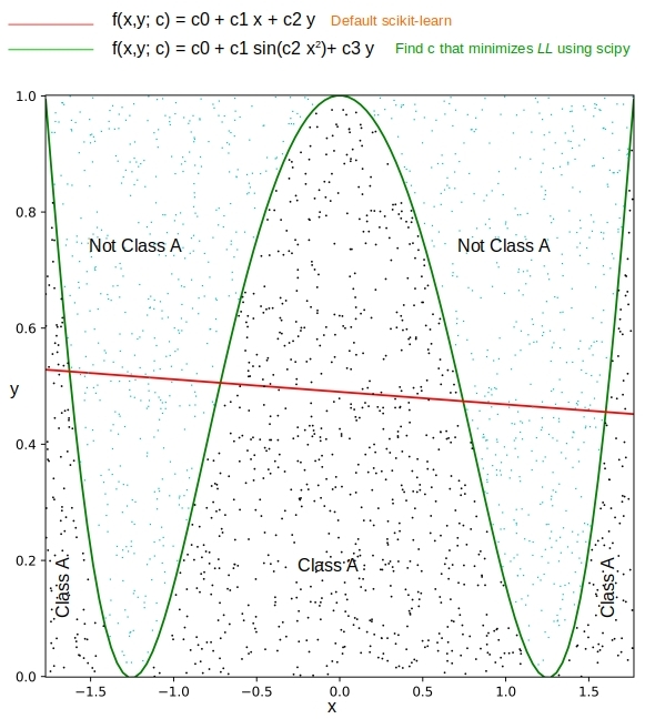
Table 2 below compares the values for the coefficients obtained in the simulation. It is interesting to note that the signs of c_1 and c_2 are opposite between the actual and those predicted by minimization. That is fine because sin(-k) = -sin(k).
| Method | c_0 | c_1 | c_2 | c_3 | F1 score |
| Actual values | 1.0 | –1.0 | 1.0 | –1.0 | |
| Find c that minimizes log(LL) | 1.0 | 1.002 | 1.0 | -0.999 | 1.0 |
| Default scikit-learn | 1.0 | -0.044 | -2.04 | 0.675 |
5. Conclusions
Logistic regression has traditionally been used to come up with a hyperplane that separates the feature space into classes. But if we suspect that the decision boundary is nonlinear we may get better results by attempting some nonlinear functional forms for the logit function. Solving for the model parameters can be more challenging but the optimization modules in scipy can help.
Hi what is different between just using a kernel method mapping the feature space using a function for say pairs of elements in the input vector? You can do this with non linear functions say like mapping x,y coordinates to an ellipse (the second order polynomial in your example) and just fit the logit to the ellipses oefficients. This way you would get the benefit of fitting your logit in a higher space and not have to drag around a kernel matrix. You would have to do extra computations at run time but you would get a higher order classifier without altering your multinomial logistic regression training function.
Chris – My understanding of kernel tricks as they are called is that they help keep the computations under control while enabling a nonlinear transformation of the features. I am not sure it applies here directly… may need changes to the formulation of the problem, I have not looked into it but is worth researching.
Here we are expanding the feature set upfront from 2 to 5 (for the 2nd degree polynomial, in 2 features). Yes, the data matrix does get larger with larger memory requirements (as number of features & degree of the polynomial increase), but is computed only once. After that it is a direct application of the out-of-the-box scikit-learn implementation. No changes there. What I was curious about though was why the prediction from scikit-learn was off a good bit (0.89 for F1 score) compared to the perfect solution (1.0 for F1) obtained by directly solving d(log(LL))/dc = 0. Thought they ought to be close to identical barring numerical issues. Any ideas on that?
Pingback: 预处理螺旋数据集以用于逻辑回归 – 学技术