Consider these two one-line documents – “Eat to Live” and “Live to Eat“. They contain the same words, but in different order – leading to a big difference in meaning. Or consider – “Working Hard” & “Hardly Working“. Popular stemmers such as snowball convert ‘Hardly‘ to ‘Hard‘ so that functionally a search engine sees two documents containing the same words. There are many such examples. Now, if a document is treated as a bag of words we cannot tell these documents apart. From an information retrieval point of view, there is no harm done. Very difficult to do, but in a conceptual clustering exercise these document pairs should perhaps not belong to the same cluster. But we are getting ahead of ourselves.
We continue here with Latent Semantic Analysis (LSA) as applied to searching and clustering of quotes. There are two types of assumptions – first in the mathematics and later in the word/meaning association that LSA makes that we need to appreciate in order to correctly interpret the results. The focus of this post is to examine some of the math and get a feel for the impact of the underlying assumptions when applied to document search and clustering. The assumptions around word/meaning association are important as well to understand, especially in the context of quotes – but that is a matter for a future post.
There are two key ideas that are central to the math of LSA. First is the vector space model (VSM) for documents – a document can be represented as a point in a term-space, where the coordinates of this point are indicative of the frequency of occurrence of those terms. The reason I say indicative is that one can normalize/scale this coordinate value in a variety of ways to improve the relevance of search results. Most, if not all search tools use VSM approach in some way, and to its great credit VSM has enabled very efficient means to find needles in haystacks. Second is the step (or a leap as some may call it) that LSA takes – causing some uneasiness given the way we think about words and documents. We will discuss this further.
1. Documents as vectors in term-space
For illustrative purposes, consider these 3 toy documents that convey the concept of urging a rabbit to escape from a fox.
- Doc 1: rabbit, fox!
- Doc 2: fox jump!
- Doc 3: run rabbit run!
The table below lists the number of occurrences of each term in each of the 3 documents
| Doc 1 | Doc 2 | Doc 3 | |
| fox | 1 | 1 | |
| jump | 1 | ||
| rabbit | 1 | 1 | |
| run | 2 |
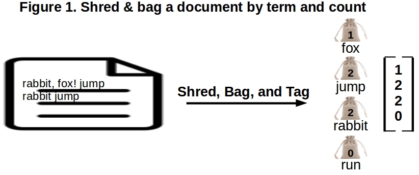
The numbers (or a variation of the same as we already mentioned) in each column are used by the VSM model to represent that document as a vector in term-space. Each term represents a dimension in this term-space. The decomposition of a document into a vector in term-space is a straightforward shred-bag-tag operation.
Given this representation of every document as a vector in term-space, a document would be considered close to an another document, if their normalized dot product is close to 1. Queries consist of terms, and so can be turned into vectors in term-space with the same shred-bag-tag operation. The search results for this query would again be those documents that have the highest dot product with this query vector. This is the gist of VSM approach.
Treating a document as a bag of words comes with its own baggage, even while it offers efficient computational means for finding needles in haystacks. We just saw that two documents can use the same set of words, and each word the same number of times – but convey a completely different meaning or describe different concepts. A couple of easy corollaries to this observation follow.
- While there is only one way we can shred-bag-tag a document, the reverse is not true.
- Given a set of terms arising from shredding a document, we can combine those terms in many ways to make many, many more documents different from the original.
2. Term-Document matrix ?
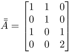
Having usefully treated each column as a 4×1 vector and gotten a lot of mileage out of it via VSM, can we go ahead now and call the above table a 4×3 matrix? It certainly looks like one, does it not? Does the arrangement of some numbers in rows and columns automatically turn that into a matrix? See a related discussion using a collaborative filtering example on Jeremy Kun’s blog. We take that plunge and write down the term-document matrix A as:
Matrix is a loaded word in linear algebra however so we need to tread with caution. But if we convince ourselves or at least appreciate the circumstances under which it can be treated as a matrix that we learnt about in linear algebra, it opens up a rich set of results that can be readily applied.
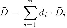
Any matrix A_mxn is by definition a linear map that operates on nx1 vectors in its domain and transforms them to mx1 vectors in its range. The domain here is the document-space with each document serving as a standard basis vector orthogonal to all other n-1 documents. The range is the term-space with each term serving as a standard basis vector orthogonal to all other m-1 terms. A point {d_1, d_2, … ,d_n} in this document-space represents a document D that is composed of d_1 number of D_1 documents, d_2 number of D_2 documents, and so forth, so we have:
Operating A_4x3 on a document with coordinates [d_1, d_2, d_3] we do get a 4×1 vector – a point in term-space for sure, but what do the new coordinate values represent?
Thus the operation of A on a document seems to be the same as the shred-bag-tag operation we depicted in Figure 1 with the VSM approach. But is this always true? Say we have a document like – “rabbit fox! run rabbit run“. We can readily shred-bag-tag it as in Figure 1 and get the vector [1, 0, 2, 2] as the term-space representation for this document. Does the operation of A on this document yield the same? Note that A can only be applied to documents in the document-space, that is only to those documents that are spanned by {D_i}. So we first should be able to locate this new document as a point in document-space and get its coordinates. It is pretty easy in this case.
We see in Figure 2 that the operation of A on this document yields exactly what we expect, the vector [1, 0, 2, 2].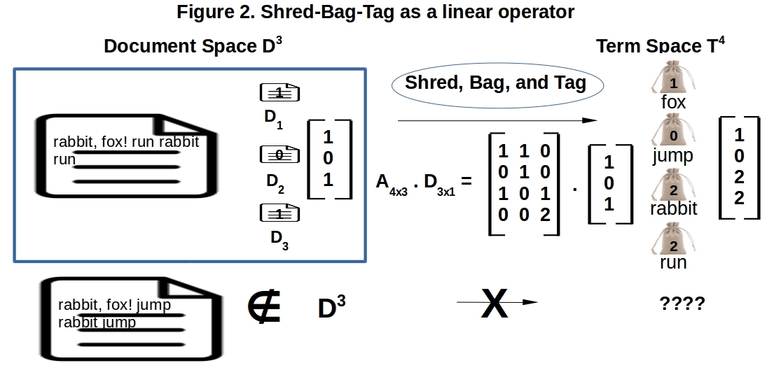
If our document cannot be located in the document-space as defined by { D_i } as the basis vectors, we would be out of luck. In other words, we can use A as a shred-bag-tag operator, if and only if we use it on documents that are in the span of { D_i } the columns of A. Our earlier document (“rabbit, fox! jump rabbit jump“) that we shred-bag-tagged for VSM is out of reach for A, as it does NOT live in the span of {D_1, D_2, D_3}. Note that VSM does not worry about a document-space, as it only needs a dot products between document vectors (or between document & query vectors) – all in term-space.
Our inability to apply A as the shred-bag-tag operator on whatever document we please is baked into the definition of A and the document-space it can operate on – no surprises there. But it is surely disconcerting in the current case where we have not introduced any new terms and the intent/concept of this new document is consistent with the other documents in the repo. We are still urging this rabbit to escape from the fox using the same set of words but in a different way. But unfortunately there is no linear operation on D_1, D_2, and D_3 documents that can ‘build’ this new document. This means that any conclusions reached by analyzing the properties of A do not apply to this new document. To be correct, we have to include this new document as a new basis vector D_4 in document-space and redo the analysis on the expanded A.
3. A quick summary
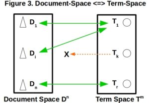
Quick summary of what we have been saying about shredding documents, document/term vector spaces and the map A between them before we start applying it in earnest to the semantic analysis of documents. This is illustrated in Figure 3 below as well.
- Document-space => Term-space is one-2-one. For any point in document-space, the operation of A yields a single point in term-space. Makes sense, as any document can be shredded & bagged in only one way – no further explanation needed.
- Range of { D_i } is a subset of Term-space. There will be points in term-space with no counterparts in document-space. Let us pick a point in term-space say [1, 0, 0, 0] which is simply 1 unit along the “fox” direction. We cannot make a document with just one “fox” term that is in the span of {D_1, D_2, D_3}. While the linearly addressable document-space is infinitely big, the space of all possible documents that can be made from the term-space is a super set, meaning that there could be a lot of similar documents that will not be under the purview of A unless they are explicitly included up-front in defining A.
- Term-space => Document-space is one-2-many. Different points in document-space can have the same image in term-space. Two documents can use the same words but in different order to convey a different meaning/idea. They are represented by a single point in term-space
Having understood some of the compromises we made in treating documents as bags words, and that table of numbers as a linear operator, we move forward with that approach. What we get in return is the ability to apply the full power of linear algebra with
and obtain useful results about documents, terms and relationships within. Before we do that let us look at a few other related matrices that will be used in deriving these results.
4. Document-Document & Term-Term affinities
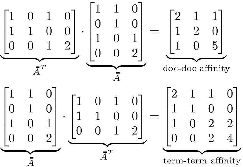
Intuitively, the documents that share a lot of terms are likely1 talking about similar topics or ideas – so we may say they have affinity to each other. And vice versa – the documents that do not have any common terms are talking about different ideas and so should have zero affinity to each other. Our document-vectors (the columns of A) are described in term-space, so the documents that have common terms will have a higher dot product compared to those that do not. The nxn matrix A^T . A, will have the dot product of i’th and j’th documents (i.e the i’th and j’th columns of ![]() ) as its element at
) as its element at ![]() . This is a doc-doc affinity matrix. In a similar fashion, the terms that appear together in documents can be considered to have more affinity to each other than those that do not – no further explanation needed. Each row of
. This is a doc-doc affinity matrix. In a similar fashion, the terms that appear together in documents can be considered to have more affinity to each other than those that do not – no further explanation needed. Each row of ![]() can be taken as the vector representation of a term in document-space. The
can be taken as the vector representation of a term in document-space. The ![]() term-term matrix
term-term matrix ![]() will have the dot product of the i’th and j’th rows of
will have the dot product of the i’th and j’th rows of ![]() , as its element at
, as its element at ![]() . This is the term-term affinity matrix.
. This is the term-term affinity matrix.
For our example in Table 1, these affinity matrices would be:
Doc 2 & Doc 3 do not share any words, so as expected we get 0 at locations ![]() and
and ![]() in the doc-doc affinity matrix. Term 1 (“fox”) and Term 4 (“run”) do not occur together in any document, so we have 0 at locations
in the doc-doc affinity matrix. Term 1 (“fox”) and Term 4 (“run”) do not occur together in any document, so we have 0 at locations ![]() and
and ![]() in the term-term affinity matrix. And so forth.
in the term-term affinity matrix. And so forth.
The point is that we can use these affinity matrices to identify the dominant relationships among documents, and among the terms – much like we do in the context of Prinicipal Component Analysis where we work with the covariance matrix built from experimental measurements on some variables. In the case of doc-doc affinity matrix, we are treating the documents as variables, and each row of ![]() as an experiment with values for each document. In the case of term-term affinity matrix we are treating the terms as variables, and each column/document as an experiment with a value for each term. Note that these affinity matrices are special. First, they are symmetric.
as an experiment with values for each document. In the case of term-term affinity matrix we are treating the terms as variables, and each column/document as an experiment with a value for each term. Note that these affinity matrices are special. First, they are symmetric.
Second, they are positive semi-definite as for any ![]()
Thereby having nice properties such as:
- real and non-negative eigenvalues that can always be written as
 where
where  is real, and
 - a full-set of orthogonal eigenvectors
The n eigenvectors of doc-doc affinity matrix ![]() can serve as an alternate basis for the document-space. The m eigenvectors of term-term affinity matrix
can serve as an alternate basis for the document-space. The m eigenvectors of term-term affinity matrix ![]() can serve as an alternate basis for the term-space. In fact we can choose the top few dominant/principal directions in each case and attempt to approximately represent the documents & terms. That is of course the whole point of talking about these affinity matrices here – to describe our stacks of documents and bags of words in terms of a few concepts that these principal directions represent! That is the subject matter for future post however.
can serve as an alternate basis for the term-space. In fact we can choose the top few dominant/principal directions in each case and attempt to approximately represent the documents & terms. That is of course the whole point of talking about these affinity matrices here – to describe our stacks of documents and bags of words in terms of a few concepts that these principal directions represent! That is the subject matter for future post however.

