The term-document matrix ![]() is a high-order, high-fidelity model for the document-space. High-fidelity in the sense that
is a high-order, high-fidelity model for the document-space. High-fidelity in the sense that ![]() will correctly shred-bag-tag it to represent it as a vector in term-space as per VSM.
will correctly shred-bag-tag it to represent it as a vector in term-space as per VSM. ![]() has
has ![]() entries, with
entries, with ![]() distinct terms (rows) building
distinct terms (rows) building ![]() documents (columns). But do we need all those
documents (columns). But do we need all those ![]() values to capture this shred-bag-tag effect of
values to capture this shred-bag-tag effect of ![]() ? That is, can we achieve it with a modified but simpler (fewer than
? That is, can we achieve it with a modified but simpler (fewer than ![]() variables) model
variables) model ![]() while accepting some error? The objective of this post is to look at a traditional approach based on the ideas in Indexing by latent semantic analysis by Deerwester et al (LSA) which is basically Singular Value Decomposition (SVD) as applied to the term-document matrix
while accepting some error? The objective of this post is to look at a traditional approach based on the ideas in Indexing by latent semantic analysis by Deerwester et al (LSA) which is basically Singular Value Decomposition (SVD) as applied to the term-document matrix ![]() . The focus is on appreciating the assumptions behind the approach, gauging the limitations that these assumptions give rise to, and interpreting the algebraic manipulations via examples.
. The focus is on appreciating the assumptions behind the approach, gauging the limitations that these assumptions give rise to, and interpreting the algebraic manipulations via examples.
1. Preliminaries
We have waded in fast and deep in the introduction above with various terminology and links. This post does build on two earlier posts Data Dimensionality and Sensitivity to Sampling and Stacks of Documents and Bags of Words in this series on text analytics. We will start with a quick summary in order to set the stage. See Figure 1 as well.
- The vector space model (VSM) represents documents as points/vectors in term-space, where the set of all distinct terms
 in the documents serve as standard basis vectors.
 - Given a set of such document vectors
 , we can form the term-document matrix
  where
where  are columns. Each column is a point/vector in term-space as per VSM.
 - While every document in the span of
 has a term-space representation, not every term in the span of
  has a representation in the document space. Clearly, the documents that can be built from a bunch of words is a superset of any finite set of documents those words may have come from.
  is a linear operator that converts any document in the span of
  to its VSM representation in term-space. The equation is:
(1) ![]()
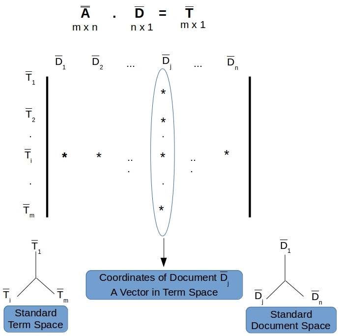
Figure 1. The term-document matrix. m rows and n columns. Each column is a VSM representation of a document in term-space.
2. Reduced Order Models
Before we embrace VSM and proceed with order reduction via SVD/LSA let us reiterate what we have bargained away by subscribing to Equation 1 as the embodiment of all truth about the documents in the repository. In words Equation1 says:
…documents are linear combinations of words…. if two documents contain the same words then they are identical… order of words, punctuation within are irrelevant… if two documents use the same words in the same proportion then they are talking about the same idea, one verbose and the other succinct…
Clearly we do not agree with the above assessments. But having started with Equation 1 as the basis for studying the properties of the repository we should temporarily put aside what text means to us and consider it as bags of words that can be processed with each bag as a variable in an equation. If we come to grips with this, the benefits are undeniable. VSM has enabled lightning fast search by keywords on large document repositories. SVD and LSA have enabled order reduction and improved search relevance by finding documents that would otherwise stay hidden by a simple keyword search alone. For example LSA can find documents that do not contain any of the supplied keywords but contain others that are related to these keywords as per the properties of ![]() .
.
Reduced order models (ROM) have been applied with reasonable success for making real-time predictions for large scale nonlinear systems such as turbulent flows. While we can apply similar techniques for reducing the dimensionality for document-spaces there is a further difference we must take note. The trouble with documents is the language itself unfortunately! Text is open to interpretation, can take different meanings based on context, and the order of words/punctuation within can drastically alter the meaning. This is unlike solving the Navier-Stokes equation which even in its full complexity has a well defined solution – provided you have specified all the boundary and initial conditions exactly. There is a mathematical certainty about physicochemical phenomena that their reduced order models can aspire to. But we do not have that luxury with documents as we do not yet know how to express the meaning of documents as deterministic functions of their ingredients. So we do the best we can at this time – take Equation 1 as the embodiment of all truth in this document repository and get the benefits that SVD and LSA offer. Thus we should not expect these reduced order models for the document repository to match/preserve the meaning of the documents but just improve search speed & relevance.
3. Dimensionality of the Document and Term Spaces
The raw document set ![]() and the raw set of distinct terms
and the raw set of distinct terms ![]() arising from them have so far been the basis vectors in their corresponding spaces. But they may not be the most advantageous bases to work with in all cases. The number of documents and terms are usually very large. If we can remove some terms/documents that do not add much new information, that is remove those terms/documents that can essentially be built from the other ones… then we can reduce the dimensionality of our system. This building of one from some others can be a linear or nonlinear operation for dimensionality reduction – but we can only deal with linear operations here. We have gone over some of this in a different post Data Dimensionality and Sensitivity to Sampling.
arising from them have so far been the basis vectors in their corresponding spaces. But they may not be the most advantageous bases to work with in all cases. The number of documents and terms are usually very large. If we can remove some terms/documents that do not add much new information, that is remove those terms/documents that can essentially be built from the other ones… then we can reduce the dimensionality of our system. This building of one from some others can be a linear or nonlinear operation for dimensionality reduction – but we can only deal with linear operations here. We have gone over some of this in a different post Data Dimensionality and Sensitivity to Sampling.
Let us say we have a document repository about movies, and the terms ‘harrison’ and ‘ford’ occur together in most cases. We can then decide to use a single compound term “harrison ford” in stead of two separate terms, thereby reducing the dimensionality of the term-space by 1. It is important to understand what we mean by occur together. We are not talking about the exact phrase like “harrison ford”. Just that, if a document contains the term “harrison” ![]() number of times, it will also contain the term “ford” about
number of times, it will also contain the term “ford” about ![]() number of times – remember the VSM model for documents. A keen reader will note that no allowance is being made for a “ford” that may have come from “gerald ford” the President, or even a ‘harrison’ from ‘george harrison’ of the Beatles fame. Let us dig into this further to clearly see the surprising reduction in dimensionality that can happen in both document and term spaces, given the VSM approach without having to apply any fancy math.
number of times – remember the VSM model for documents. A keen reader will note that no allowance is being made for a “ford” that may have come from “gerald ford” the President, or even a ‘harrison’ from ‘george harrison’ of the Beatles fame. Let us dig into this further to clearly see the surprising reduction in dimensionality that can happen in both document and term spaces, given the VSM approach without having to apply any fancy math.
Example 1. Of Harrisons & Fords!
Consider the following three documents which we know to be different, thus expecting a dimension of 3 for the document-space. But VSM thinks otherwise and says the dimension is 1. In the first document Harrison Ford is being asked to watch over a couple of kids as they played. In the second, President Ford watched a performance from George Harrison. And in the third, President Ford and Harrison Ford watched a play while George Harrison played with the same kids.
- Watch Gerald and George at Play, Harrison Ford!
- Gerald Ford Watched a Play by George Harrison
- Harrison Ford and Gerald Ford Watched a Play while George Harrison Played with Gerald and George
You may complain that I am just playing on words, but these documents are describing different things as we understand them. But from the VSM perspective, Doc 1 and Doc 2 are the same, and Doc 3 is simply a linear combination of the first two. The 6-dimensional term-space basis is:
(2) ![]()
And the document vectors are:
(3) 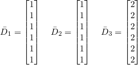
Thus as per VSM there is only one real document here and the dimensionality of the document-space is 1. Given such a one-dimensional document-space we can use just one compound term “ford george gerald harrison play watch” in stead of six terms for the term-space, and that would be sufficient to model all the documents in this document-space. Unsatisfactory state-of-affairs it may seem as the meaning of the sentences got lost while getting shredded, but we did get a massive dimensionality reduction if that is any comfort!. But this is a repository of movies and President Ford or Mr. Harrison were not movie actors as far as I know to be masquerading as Harrison Ford in the document repo, and so unlikely to happen.
3.1 Principal Component Analysis
While we can eyeball these dimensionality-reducing compound terms, or even documents that are linear combinations of other documents when the repository is small – it is impractical for large repos. In fact, we want to use the fewest number of these compounded terms that can adequately describe all the documents in the repo. The rigorous way of identifying these linearly compounded terms that can be helpful in reducing the dimensionality of the term-space is of course known from Principal Component Analysis. The eigenvectors of the term-term affinity matrix turn out to be these compound terms. We know that eigenvectors in term-space are simply linear combinations of the original discrete terms – much like the commonly occurring compound terms we had eyeballed for. Further, the eigenvectors with the largest eigenvalues are the most dominant compound terms to be found across all the documents in the repo. This discussion applies equally from the point of view of documents as well, leading to the conclusion that the eigenvectors of the document-document affinity matrix are the compound documents one could use as a dimensionality-reducing basis for the document-space.
So if we are limited to say using only ![]() (much smaller than
(much smaller than ![]() or
or ![]() ) dimensions, we would pick the first
) dimensions, we would pick the first ![]() number of these eigenvectors arranged as per their decreasing eigenvalues to get the best approximation in each semantic-space. That is the basic idea behind Indexing by latent semantic analysis by Deerwester et al borrowed from Singular Value Decomposition (SVD) as applied to the term-document matrix.
number of these eigenvectors arranged as per their decreasing eigenvalues to get the best approximation in each semantic-space. That is the basic idea behind Indexing by latent semantic analysis by Deerwester et al borrowed from Singular Value Decomposition (SVD) as applied to the term-document matrix.
3.2 Rank of 
We will conclude this section with a couple of notes about the rank of the term-document matrix in Equation 1. The rank ![]() of
of ![]() is the maximum size of the dimensionality we had been after in the above discussion.
is the maximum size of the dimensionality we had been after in the above discussion.
 cannot be greater than the minimum of
  and
and  .
.- The
 terms are the distinct terms obtained by shredding the documents. In reverse, all
  documents (and more!) can be linearly built from these
  terms – no explanation needed. So the number of independent documents
  can never be greater than
  . We went over this in the earlier post Stacks of Documents and Bags of Words where we described the span of document-space being a subset of the all the documents that can built from the individual terms.
So we have the rank ![]() of
of ![]() as the number of linearly independent documents.
as the number of linearly independent documents.
Example 2
Consider the two documents where we are unsuccessfully trying to get our dog to exercise.
- fetch dog fetch!
- lazy dog!
They are linearly independent. ![]() is 2, that is the document-space is 2-dimensional. The number of distinct terms
is 2, that is the document-space is 2-dimensional. The number of distinct terms ![]() that these two documents contain is 3, so the term-space is 3-dimensional. But the rank of
that these two documents contain is 3, so the term-space is 3-dimensional. But the rank of ![]() is 2.
is 2.
Example 3
Consider the three documents where you are urging a rabbit to escape from a fox.
- fox!
- rabbit, fox!
- run rabbit run! fox!
Both the document and term spaces are 3-dimensional and the rank of ![]() is 3.
is 3.
4. Document-Document and Term-Term Affinities
The affinity between the documents (as per their VSM representations in the term-space of course) is given by the matrix ![]() . Likewise, the affinity between the terms is given by the matrix
. Likewise, the affinity between the terms is given by the matrix ![]() . On account of being real and symmetric, they both have eigen decompositions.
. On account of being real and symmetric, they both have eigen decompositions.
(4) ![]()
(5) ![]()
![]() is the diagonal matrix with real, non-negative eigenvalues – hence the use of a square value to indicate this. The fact that both
is the diagonal matrix with real, non-negative eigenvalues – hence the use of a square value to indicate this. The fact that both ![]() and
and ![]() have the same non-zero eigenvalues is a basic result in linear algebra1. With no loss of generality the
have the same non-zero eigenvalues is a basic result in linear algebra1. With no loss of generality the ![]() are arranged in decreasing order as in:
are arranged in decreasing order as in:
(6) ![]()
And as per our discussion about the rank of ![]() ,
,
(7) ![]()
![]() is the column matrix of
is the column matrix of ![]() orthonormal eigenvectors in document-space.
orthonormal eigenvectors in document-space. ![]() is the column matrix of
is the column matrix of ![]() orthonormal eigenvectors in term-space. That is, with
orthonormal eigenvectors in term-space. That is, with ![]() as the identity matrix,
as the identity matrix,
(8) 
Time for an example to convince ourselves of what we started this section with – how the eigenvectors of the affinity matrices allow us to automatically come up with compound terms/documents that can reduce the dimensionality of the corresponding spaces.
Example 4
Consider the following four documents where we are urging a rabbit to escape from the fox, and unsuccessfully urging the dog to save the rabbit from this fox.
 : run dog! fox is jumping in! rabbit run!
 : dog, jump on fox!
 : run rabbit run!
 : fox is running with the rabbit! run lazy dog jump!
The standard ordered basis for the term-space are the six distinct terms ![]() . A bit more difficult to eyeball but the following terms occur together in the indicated ratios whenever any one of them is present in a document.
. A bit more difficult to eyeball but the following terms occur together in the indicated ratios whenever any one of them is present in a document.
(9) ![]()
And, the first document is a simple addition of the second and third documents. That is:
(10) ![]()
From Equation 9 we know that we should be able to just use 3 terms to describe the document-space and be none the worse for it. Those three terms being: (a) one compound term in place of the 3 terms ![]() , (b) another compound term in place of the 2 terms
, (b) another compound term in place of the 2 terms ![]() , and (c) the regular term
, and (c) the regular term ![]() . And from Equation 10 we know that we only have 3 independent documents. Three compound terms completely describing 3 documents – a rank of 3 for the term-document matrix.
. And from Equation 10 we know that we only have 3 independent documents. Three compound terms completely describing 3 documents – a rank of 3 for the term-document matrix.
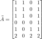
Now we shall verify if all the algebra in this section agrees with our intuitive assessments above.The term-document matrix is ![]() is:
is:
(11) 
The term-term affinity matrix and its eigen decomposition can be readily computed. The eigenvalues turn out to be,
(12) ![]()
confirming that the rank of ![]() is 3 – perfect! The corresponding 3 eigenvectors in term-space (we do not care for the other 3 as their eigenvalues are zero) are:
is 3 – perfect! The corresponding 3 eigenvectors in term-space (we do not care for the other 3 as their eigenvalues are zero) are:
(13) 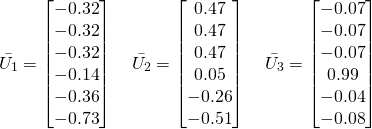
The first three values in these vectors are the weights for the terms ![]() and the last two are the weights for the terms
and the last two are the weights for the terms ![]() . Rewriting them as 3-dimensional vectors allows us to see our compound terms at play confirming our intuitive assessment.
. Rewriting them as 3-dimensional vectors allows us to see our compound terms at play confirming our intuitive assessment.
(14) 
Before leaving this example we note the eigenvectors ![]() of the document-document affinity matrix. We will be using them in the coming sections as the basis for document-space.
of the document-document affinity matrix. We will be using them in the coming sections as the basis for document-space.
(15) 
5. The Relation Between eigen documents and eigen terms
We have stated that our goal was to use the document-space eigenvectors ![]() as the basis for document-space and the term-space eigenvectors
as the basis for document-space and the term-space eigenvectors ![]() as the basis for term-space.
as the basis for term-space. ![]() is simply a compound term that is a linear combination of the discrete terms as we have just seen in Example 4. Likewise
is simply a compound term that is a linear combination of the discrete terms as we have just seen in Example 4. Likewise ![]() is a compound document that is a linear combination of the standard basis documents. And most importantly, it turns out that
is a compound document that is a linear combination of the standard basis documents. And most importantly, it turns out that ![]() and
and ![]() are related in a natural way – this is the crux of SVD.
are related in a natural way – this is the crux of SVD.
5.1.  is an orthonormal set in term-space
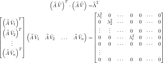
If we are going to express documents with ![]() as the basis, we need to first understand what our shred-bag-tag operator (Equation 1) will do to these eigen/compound documents. That is, what is
as the basis, we need to first understand what our shred-bag-tag operator (Equation 1) will do to these eigen/compound documents. That is, what is ![]() ? To see that let us rewrite 4 as:
? To see that let us rewrite 4 as:
(16) 
(17) 
As the rank ![]() we know that we will have
we know that we will have ![]() rows & columns of zeros in the diagonal matrix
rows & columns of zeros in the diagonal matrix ![]() . So we only need to consider the first
. So we only need to consider the first ![]() columns of
columns of ![]() (or
(or ![]() ).
).
From Equations 6 and 7 we have ![]() so we can rewrite Equation 17 for
so we can rewrite Equation 17 for ![]() as:
as:
(18) 
Equations 17 and 18 tell us that the ![]() vectors
vectors ![]() are an orthonormal set in term-space. So they can very well serve as the basis for the image/range of
are an orthonormal set in term-space. So they can very well serve as the basis for the image/range of ![]() in term-space as the rank of
in term-space as the rank of ![]() is
is ![]() .
.
But so what? In any given space there are infinitely many orthonormal bases. What is so special about these ![]() orthonormal vectors
orthonormal vectors ![]() in the term-space? It turns out these are not any orthonormal basis vectors, but the same as the term-space eigenvectors
in the term-space? It turns out these are not any orthonormal basis vectors, but the same as the term-space eigenvectors ![]() that have simply been scaled. This is of course the jewel crown of an observation from Singular Value Decomposition (SVD) proved below.
that have simply been scaled. This is of course the jewel crown of an observation from Singular Value Decomposition (SVD) proved below.
5.2. Shred-Bag-Tag operation on an eigen document turns it into a scaled eigen term.
We can see this by left multiplying ![]() with
with ![]() .
.
(19) 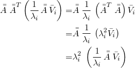
The last equality in Equation 19 above shows that ![]() is an eigenvector of
is an eigenvector of ![]() with the eigenvalue
with the eigenvalue ![]() . We had been calling that
. We had been calling that ![]() all this time. Thus the core result of SVD in scalar form:
all this time. Thus the core result of SVD in scalar form:
(20) ![]()
Grouping the eigenvectors, we get the more familiar matrix form for SVD:
(21) 
Example 4 (continued)
We return to our lazy dog example to see whether the eigenvectors ![]() we obtained do in fact obey Equation 20. Take
we obtained do in fact obey Equation 20. Take ![]() for example:
for example:
![Rendered by QuickLaTeX.com \[ \Bar{\Bar{A}} \; \Bar{V}_1 = \begin{bmatrix} 1 & 1 & 0 & 1 \\ 1 & 1 & 0 & 1 \\ 1 & 1 & 0 & 1 \\ 0 & 0 & 0 & 1 \\ 1 & 0 & 1 & 1 \\ 2 & 0 & 2 & 2 \end{bmatrix} \; \begin{bmatrix} -0.61 \\ -0.21 \\ -0.4 \\ -0.65 \end{bmatrix} = \begin{bmatrix} -1.47 \\ -1.47 \\ -1.47 \\ -0.65 \\ -1.66 \\ -3.32 \end{bmatrix} = \frac{1}{4.55} \begin{bmatrix} -0.32 \\ -0.32 \\ -0.32\\ -0.14 \\ -0.36 \\ -0.73 \end{bmatrix} = \frac{1}{\lambda_1} \; \Bar{U}_1 \]](https://xplordat.com/wp-content/ql-cache/quicklatex.com-0e2caf5fdd2b2003d5847760b5fe028f_l3.png)
Thus agreeing with Equation 20 .
6. Reduced Order Models for Documents
The main driver for this article has been the anticipated reduction in the number of documents/terms we need to consider in capturing the essence of the full document repository. From all the analysis in the earlier sections we have the tools now to identify the dominant compound terms and we are going to test them against our lazy dog example.
When we consider only the first ![]() compound terms (
compound terms (![]() ), in Equation 21, the term-document matrix
), in Equation 21, the term-document matrix ![]() can be approximated as
can be approximated as ![]() :
:
(22) 
We will apply this to Example 4 for which we have already computed all the needed eigenvectors & eigenvalues. We know that the rank is 3. So the maximum number of eigenvectors we need to consider is 3. That is we should get ![]() to be identical to
to be identical to ![]() , with
, with ![]() and
and ![]() faring progressively worse. But how worse? Let us do this with a quick python script.
faring progressively worse. But how worse? Let us do this with a quick python script.
|
1 2 3 4 5 6 7 8 9 10 11 12 13 14 15 16 17 18 19 20 21 22 23 24 25 26 27 28 29 30 31 32 33 34 35 36 37 38 39 40 41 |
import numpy as np import numpy.linalg as linalg np.set_printoptions(precision=2,suppress=True) # Documents: # D_1: run dog! fox is jumping in! rabbit run! # D_2: dog, jump on fox! # D_3: run rabbit run! # D_4: fox is jumping on rabbit! run you lazy dog run! # Terms: # dog, fox, jump, lazy, rabbit, run A = np.array([ [1,1,0,1], [1,1,0,1], [1,1,0,1], [0,0,0,1], [1,0,1,1], [2,0,2,2] ]) U, s, VT = np.linalg.svd(A, full_matrices=True) D = np.diag(s) # augment D with extra rows/columns of zeroes as needed m = U.shape[0] n = VT.shape[0] if (m > n): extra_rows = m - n for i in range (0, extra_rows): D = np.vstack((D,np.zeros(n))) else: extra_cols = n - m for i in range (0, extra_cols): D = np.vstack((D,np.zeros(m))) # Reduced order models. # Test Document D_2 + D_3 : dog, run over fox! run rabbit, jump! testDocument = np.array([0,1,1,0]).reshape(4, 1) pLimits = [3, 2, 1] for p in pLimits: Up = U[:,0:p] Dp = D[0:p,0:p] VTp = VT[0:p,:] UpDp = np.matmul(Up, Dp) Ap = np.matmul(UpDp, VTp) print ('p = ',p) print (Ap) print ('Frobenius Norm:',np.linalg.norm(Ap)) print (np.matmul(Ap, testDocument)) |
Running which we get ![]() to be identical to
to be identical to ![]() as expected and other two showing some deviations.
as expected and other two showing some deviations.
![Rendered by QuickLaTeX.com \[ {\Bar{\Bar{A}}}_3 = \begin{bmatrix} 1 & 1 & 0 & 1 \\ 1 & 1 & 0 & 1 \\ 1 & 1 & 0 & 1 \\ 0 & 0 & 0 & 1 \\ 1 & 0 & 1 & 1 \\ 2 & 0 & 2 & 2 \end{bmatrix} {\Bar{\Bar{A}}}_2 = \begin{bmatrix} 0.97 & 0.98 & -0.01 & 1.04 \\ 0.97 & 0.98 & -0.01 & 1.04 \\ 0.97 & 0.98 & -0.01 & 1.04 \\ 0.4 & 0.21 & 0.19 & 0.43 \\ 0.98 & -0.01 & 0.99 & 1.02 \\ 1.97 & -0.02 & 1.98 & 2.05 \end{bmatrix} {\Bar{\Bar{A}}}_1 = \begin{bmatrix} 0.9 & 0.31 & 0.59 & 0.95 \\ 0.9 & 0.31 & 0.59 & 0.95 \\ 0.9 & 0.31 & 0.59 & 0.95 \\ 0.4 & 0.14 & 0.26 & 0.42 \\ 1.02 & 0.35 & 0.67 & 1.07 \\ 2.04 & 0.71 & 1.33 & 2.14 \end{bmatrix} \]](https://xplordat.com/wp-content/ql-cache/quicklatex.com-ef631a599f3ed66ce43c6f64eecb2de2_l3.png)
Defining a relative distance/error measure using the Frobenius norm for matrices as,
(23) 
we get:
(24) ![]()
indicating that if we can live with 15% error for the shred-bag-tag operation, we can cut down the number of variables to work with from 24 (4 docs with 6 terms each) variables, to 9 (3 eigen docs with 3 eigen terms each). But the real measure of error is what ![]() does to a document. Take a test document
does to a document. Take a test document
![]()
It is in the span of ![]() as it is simply
as it is simply ![]() . Operating
. Operating ![]() on
on ![]() we get the term-space representations as:
we get the term-space representations as:
(25) 
Except for the ![]() term the match for the rest is not bad, even with one compound term.
term the match for the rest is not bad, even with one compound term.
7. Next Steps
This was a long post unfortunately but mainly due to the examples and it just would not do to break them up. But we have made a lot of progress towards a semantic analysis of documents. We have obtained sets of terms that are observed to occur together among the documents in the repository. When we find a frequent juxtaposition of the same terms across documents, or many places in the same document – the documents are likely describing the same mini-concept, one of the core assumptions behind a semantic analysis of text. The document repository is then taken to be made up of these identified concepts. This allows for extra insights than what a simple keyword based search can provide. And, opens doors to relate & cluster the documents by concepts. We will get into the details in the next article in this series.
- see Gilbert Strang for example

