For generic text, word bag approaches are very efficient at text classification. For a binary text classification task studied here, LSTM working with word sequences is on par in quality with SVM using tf-idf vectors. But performance is a different matter…
The bag-of-words approach to turning documents into numerical vectors ignores the sequence of words in the documents. Classifiers that work off of such vectors are then expected to pay the price for not accounting for the difference a specific sequence of words makes to the meaning and the implied target class thereof. Makes sense. That is the argument anyways in considering the newer deep learning approaches such as LSTM (Long Short-Term Memory) neural nets that can work with sequences. In the previous article we have indeed shown that the naive bayes classifier using word bag vectors (tf-idf to be specific) took a drubbing in the hands of LSTM (0.23 for naive-bayes/tf-idf vs 0.91 with LSTM for the F1-score) when the sequence of words was the deciding the factor for classification.
But that text corpus was artificial. It was constructed to bring out the best in sequence respecting models such as LSTM and the worst in others that ignored the said sequence at their peril. Does this out performance on the part of LSTM extend to a real life text corpus where the sequence of words may not be the deciding factor for classification? That is the question we explore here. We start with a simpler binary classification task in this post and consider a multilabel classification task in a later post. We use Support Vector Machines (SVM) with tf-idf vectors as the proxy for bag-of-words approach and LSTM for the sequence respecting approach. SVM is implemented via SciKit and LSTM is implemented via Keras. While we go through some code snippets here, the full code for reproducing the results can be downloaded from github.
1. Tokenize the Movie Reviews
The text corpus, large movie reviews from Stanford is often used for binary sentiment classification – i.e. is the movie good or bad based on the reviews. The positive and negative reviews are downloaded to disk in separate directories. Here is the code snippet to ‘clean’ the documents and tokenize them for analysis.
# Read the Text Corpus, Clean and Tokenize
import numpy as np
from nltk.tokenize import RegexpTokenizer
from nltk.corpus import stopwords
from sklearn.datasets import fetch_20newsgroups
nltk_stopw = stopwords.words('english')

def tokenize (text):        #   no punctuation & starts with a letter & between 2-15 characters in length
    tokens = [word.strip(string.punctuation) for word in RegexpTokenizer(r'\b[a-zA-Z][a-zA-Z0-9]{2,14}\b').tokenize(text)]
    return  [f.lower() for f in tokens if f and f.lower() not in nltk_stopw]

def getMovies():
    X, labels, labelToName  = [], [], { 0 : 'neg', 1: 'pos' }
    for dataset in ['train', 'test']:
        for classIndex, directory in enumerate(['neg', 'pos']):
            dirName = './data/' + dataset + "/" + directory
            for reviewFile in os.listdir(dirName):
                with open (dirName + '/' + reviewFile, 'r') as f:
                    tokens = tokenize (f.read())
                    if (len(tokens) == 0):
                        continue
                X.append(tokens)
                labels.append(classIndex)
    nTokens = [len(x) for x in X]
return X, np.array(labels), labelToName, nTokens- Lines #10 – 11. Tokenization. Remove all punctuation and NLTK stop words. Make sure all words/tokens start with a letter. And only retain those words between 3 and 15 characters long.
- Line #15 – 24: Loop through the movie review files in each folder and tokenize.
- Line # 25: Taking note of number of words in each document helps us choose a reasonable sequence length for LSTM later. The percentile stats on nTokens shows that over 86% of the documents have less than 200 words in them.
Token Summary:
min  avg    median   std     85/86/87/90/95/99         max
3    116      86      88    189/195/203/230/302/457    1388
2. Pack Bags and Sequences
LSTM works with word sequences as input while the traditional classifiers work with word bags such as tf-idf vectors. Having each document in hand as a list of tokens we are ready for either.
2.1 Tf-Idf Vectors for SVM
We use Scikit’s Tf-Idf Vectorizer to build the vocabulary and the document vectors from the tokens.
# Build Tf-Idf Vectors
from sklearn.feature_extraction.text import TfidfVectorizer
X=np.array([np.array(xi) for xi in X]) # rows:Docs. columns:words
vectorizer = TfidfVectorizer(analyzer=lambda x: x, min_df=1).fit(X)
word_index = vectorizer.vocabulary_
Xencoded = vectorizer.transform(X)
2.2 Sequences for LSTM
The text processor in Keras turns each document into a sequence/string of integers, where the integer value indicates the actual word as per the {word:index} dictionary that the same processing generates. We use 200-long sequences as the stats on the tokens show that over 86% of the documents have less than 200 words. In Line # 8 in the code below, the documents with fewer than 200 words will be ‘post’ padded with the index value 0 that is ignored by the embedding layer (mask_zero=True is set for in the definition of embedding layer in Section 3).
# Turn text into 200-long integer sequences, padding with 0 if necessary to maintain the length at 200
import keras
sequenceLength = 200
kTokenizer = keras.preprocessing.text.Tokenizer()
kTokenizer.fit_on_texts(X)
encoded_docs = kTokenizer.texts_to_sequences(X)
Xencoded = keras.preprocessing.sequence.pad_sequences(encoded_docs, maxlen=sequenceLength, padding='post')
3. Models
LSTM is implemented via Keras while SVM is implemented via SciKit. Both work with the same train/test split so a comparison would be fair. Twenty percent of the overall corpus (i.e 10,000 documents) are set aside for test while training on the remaining 40,000 documents.
# Test/Train Split
from sklearn.model_selection import StratifiedShuffleSplit
sss = StratifiedShuffleSplit(n_splits=1, test_size=0.2, random_state=1).split(Xencoded, labels)
train_indices, test_indices = next(sss)
train_x, test_x = Xencoded[train_indices], Xencoded[test_indices]
3.1 LSTM
As in the earlier article, we use the simplest possible LSTM model, with an embedding layer, one LSTM layer and the output layer.

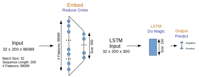
The embedding layer in Figure 1 reduces the number of features from 98089 (the number of unique words in the corpus) to 300. The LSTM layer outputs a 150-long vector that is fed to the output layer for classification. The model itself is defined quite simply below.
- Line #4: Embedding layer is trained to convert the 98089 long 1-hot vetcors to dense 300-long vectors
- Line #6: The dropout fields are to help with preventing overfitting
# A Simple Model for LSTM
model = keras.models.Sequential()
embedding = keras.layers.embeddings.Embedding(input_dim=len(kTokenizer.word_index)+1, output_dim=300, input_length=sequenceLength, trainable=True, mask_zero=True)
model.add(embedding)
model.add(keras.layers.LSTM(units=150, dropout=0.2, recurrent_dropout=0.2, return_sequences=False))
model.add(keras.layers.Dense(numClasses, activation='softmax'))
model.compile(optimizer='adam', loss='categorical_crossentropy', metrics=['acc'])
print(model.summary())
Training is done with early stopping to prevent over training in Line #6 in the code below. The final output layer yields a vector that is as long as the number of labels, and the argmax of that vector is the predicted class label.
# Train and Predict with LSTM
train_labels = keras.utils.to_categorical(labels[train_indices], len(labelToName))
test_labels = keras.utils.to_categorical(labels[test_indices], len(labelToName))
early_stop = keras.callbacks.EarlyStopping(monitor='val_loss', min_delta=0, patience=5, verbose=2, mode='auto', restore_best_weights=False)
history = model.fit(x=train_x, y=train_labels, epochs=50, batch_size=32, shuffle=True, validation_data = (test_x, test_labels), verbose=2, callbacks=[early_stop])
predicted = model.predict(test_x, verbose=2)
predicted_labels = predicted.argmax(axis=1)
3.2 SVM
The model for SVM is much less involved as there are far fewer moving parts and parameters to decide upon. That is always a good thing of course.
# Train and Predict with SVM
from sklearn.svm import LinearSVC
model = LinearSVC(tol=1.0e-6,max_iter=5000,verbose=1)
train_labels = labels[train_indices]
test_labels = labels[test_indices]
model.fit(train_x, train_labels)
predicted_labels = model.predict(test_x)
4. Simulations
The confusion matrix and the F1-scores obtained are what we are interested in. With the predicted labels in hand from either approach we use SciKit’s API to compute them.
# Get Confusion Matrix and Classification Report
from sklearn.metrics import classification_report, confusion_matrix
print (confusion_matrix(labels[test_indices], predicted_labels))
print (classification_report(labels[test_indices], predicted_labels, digits=4, target_names=namesInLabelOrder))
While we have gone through some snippets in different order, the complete code for lstm_movies.py for running LSTM and svm_movies.py for running SVM is on github. As indicated in the previous article, various random seeds are initialized for repeatability.
4.1 LSTM
Running LSTM with:
#!/bin/bash

echo "PYTHONHASHSEED=0 ; pipenv run python ./lstm_movies.py"
PYTHONHASHSEED=0 ; pipenv run python ./lstm_movies.py
yields about 0.87 as the F1-score converging in 6 epochs due to early stopping.
Using TensorFlow backend.
Token Summary:min/avg/median/std 85/86/87/88/89/90/95/99/max:
3 116.47778 86.0 88.1847205941687 189.0 195.0 203.0 211.0 220.0 230.0 302.0 457.0 1388
X, labels #classes classes 50000 (50000,) 2 ['neg', 'pos']
Vocab padded_docs 98089 (50000, 200)
_________________________________________________________________
Layer (type)                 Output Shape              Param #
=================================================================
embedding_1 (Embedding)      (None, 200, 300)          29427000
_________________________________________________________________
lstm_1 (LSTM)                (None, 150)               270600
_________________________________________________________________
dense_1 (Dense)              (None, 2)                 302
=================================================================
Total params: 29,697,902
Trainable params: 29,697,902
Non-trainable params: 0
_________________________________________________________________
None
Train on 40000 samples, validate on 10000 samples
Epoch 1/50
 - 1197s - loss: 0.3744 - acc: 0.8409 - val_loss: 0.3081 - val_acc: 0.8822
Epoch 2/50
 - 1195s - loss: 0.1955 - acc: 0.9254 - val_loss: 0.4053 - val_acc: 0.8337
...
Epoch 6/50
 - 1195s - loss: 0.0189 - acc: 0.9938 - val_loss: 0.5673 - val_acc: 0.8707
Epoch 00006: early stopping
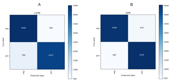
[[4506  494]
 [ 799 4201]]
              precision    recall  f1-score   support

         neg     0.8494    0.9012    0.8745      5000
         pos     0.8948    0.8402    0.8666      5000

   micro avg     0.8707    0.8707    0.8707     10000
   macro avg     0.8721    0.8707    0.8706     10000
weighted avg     0.8721    0.8707    0.8706     10000

Time Taken: 7279.333829402924
4.2 SVM
Running SVM with
#!/bin/bash

echo "PYTHONHASHSEED=0 ; pipenv run python ./svm_movies.py"
PYTHONHASHSEED=0 ; pipenv run python ./svm_movies.py
yields 0.90 as the F1-score
Token Summary. min/avg/median/std/85/86/87/88/89/90/95/99/max:
3 116.47778 86.0 88.1847205941687 189.0 195.0 203.0 211.0 220.0 230.0 302.0 457.0 1388
X, labels #classes classes 50000 (50000,) 2 ['neg', 'pos']
Vocab sparse-Xencoded 98089 (50000, 98089)
.....*
optimization finished, #iter = 59
Objective value = -6962.923784
nSV = 20647
[LibLinear][[4466  534]
 [ 465 4535]]
              precision    recall  f1-score   support

         neg     0.9057    0.8932    0.8994      5000
         pos     0.8947    0.9070    0.9008      5000

   micro avg     0.9001    0.9001    0.9001     10000
   macro avg     0.9002    0.9001    0.9001     10000
weighted avg     0.9002    0.9001    0.9001     10000

Time Taken: 0.7256226539611816
5. Conclusions
Clearly, both SVM at 0.90 as the F1-score and LSTM at 0.87 have done very well for binary classification. The confusion matrices show excellent diagonal dominance as expected.

While they are equal on the quality side, LSTM does take much longer – 2hrs as opposed to less than a second. That is too big a difference to be ignored.
With that we conclude this post. In the next post we go over the results for a multilabel classification exercise and the impact of external word-embeddings such as fasttext.

For this code, how to add word embedding process with three args none,fasttext and custom?
It would be essentially identical to the code in the other article. The ‘none’ case is already here. For the ‘custon’ case you need to generate the word-embeddings. You can use GenSim for that. The other article
http://xplordat.com/2018/10/09/word-embeddings-and-document-vectors-part-2-classification/
has details on how to generate custom word vectors with Gensim