Formulae for trainable parameter counts are developed for a few popular layers as function of layer parameters and input characteristics. The results are then reconciled with what Keras reports upon running the model…
Deep learning models are parameter happy. Safe to say they have never met a parameter they did not like! Models employing millions of parameters are all too common and some run into billions as well. Thanks to low level libraries such as TensorFlow, PyTorch etc… for the heavy lifting and high level libraries such as Keras for ease of use, it is easy to rapidly build such models now-a-days. But knowing how these parameters come about from the fundamentals is important to go beyond a blackbox approach to deep learning. That is the objective of this post – perhaps can help someone with an interview question or two for a deep learning engineer role!
A most useful output from running Keras is the shape of data/tensors entering/leaving each layer and the count of trainable parameters in that layer. For regular practitioners of deep learning, this information is a quick confirmation that Keras is running what they programmed it for. But for those new to deep learning, it may not be immediately clear as to how these come about. Here we look at the inner workings of some popular layers, not too deep but just enough to derive the number of parameters as a function of the layer parameters. And we reconcile the same with what Keras tells us there to be. Here is a brief outline.
- Pick some frequently layers such as Dense, Embedding, RNN (LSTM/GRU), and Convolutions (Conv1D/Conv2D) etc… Due to length concerns we will take up Convolutions in the next post in this series.
- For each layer, develop formulae for the number of trainable parameters as a function of the layer specific details such as the number of units, filters and their sizes, padding etc… and input details such as the number of features, channels etc… We further obtain the expected shape of the data/tensor leaving the layer
- Run the Video question answering model described in Keras guide and confirm that our formulae/analysis is correct for the trainable parameters and the output shapes.
The complete code for the snippets shown here can be downloaded from github as usual.
1. Layers galore
A deep learning model is a network of connected layers with each layer taking an input data tensor and generating an output data tensor of potentially different shape. Each layer uses a tonne of parameters to do its job, adding to the overall number of parameters in the model. The data/tensors flow across the network from input(s) to output(s) while getting transformed in shape and content along the way. The model parameters are estimated in the training phase by comparing the obtained and expected outputs and then driving the error backwards to update these parameters so they would do better for the next batch of inputs. That is deep learning in a nut shell – just a massive optimization exercise in a billion dimensional space!
Keras provides high level API for instantiating a variety of layers and connecting them to build deep learning models. All the computation happens inside these layers. Popular layers include the ‘bread and butter’ Dense layer, ‘image happy’ Convolutional layers, ‘sequence respecting’ Recurrent layers and many variations thereof. There are functional layers such as pooling that do not add new parameters but change the shape of the incoming tensor. There are normalization layers that do not modify the shape but add new parameters. There are layers like dropout that neither add new parameters nor modify the shape. You get the point – there is layer for it! Besides we can write custom layers as well. For our purposes we just focus on a few popular layers. First some definition and notation.
A tensor is simply a multidimensional matrix of numbers with an arbitrary shape like [n_1, n_2, n_3, …n_m]. A vector is a list of numbers and so has one dimension like [n_1]. Clearly a vector is a tensor with one dimension. We choose however to write a vector as [n_1,1] to emphasize that it is just a matrix with one column and to see that all dot and hadamard products work out cleanly.
2. Dense layer
Dense layers are the building blocks of simple feed forward networks. Each input is connected to every unit in the layer, and each such connection has an associated weight. Plus each unit has a bias (if use_bias=True in Keras, the default) . Equation 1 below captures what a dense layer does. Based on a choosable activation function f, it simply transforms the input vector x to an output vector y.
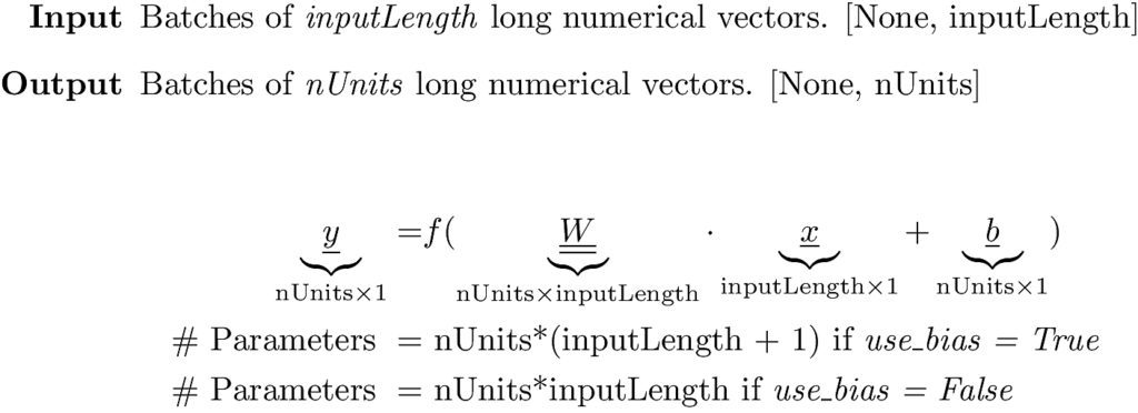
For example he following model will have 32 * (784 +1) = 25120 trainable parameters verified by running the model.
model = Sequential()
# use_bias=True by default
model.add(Dense(units=32, input_shape=(784,), name='Dense_Layer'))
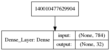
Running which we get the following output and data flow graph.
Layer (type)                 Output Shape              Param #
=================================================================
Dense_Layer (Dense)          (None, 32)                25120
=================================================================
Total params: 25,120
Trainable params: 25,120
Non-trainable params: 0
3. Embedding layer
Embedding layers are almost identical to dense layers but very important to talk about as they are extensively used in preparing text input.
An embedding layer is a dense layer without bias parameters and identity as the activation function. In fact all the layer does is a matrix multiply where the matrix entries are learnt during training
Embedding layers are used in text processing to come up with numerical vector representations of words. The words making up the text corpus are assigned integer indices starting at 0 (or 1 if 0 is being used for padding/masking in order to allow for variable length sentences) through nWords (or nWords+1 if 0 is used for masking). The input sentence/text has at most sequenceLength words. Each word is a 1-hot encoded vector. The weight matrix converts a long 1-hot encoded vector to a short dense numerical vector. In other words the weight matrix is simply the word-vectors as columns of length nUnits.
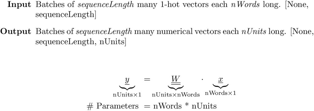
The following code snippet for an embedding layer would add 1024 * 256 = 262144 trainable parameters to the model matching with what Keras reports below.
nWords = 1024
sequence_length = 25
model = Sequential()
model.add(Embedding(input_dim=nWords, output_dim=256, input_length=sequence_length, name='Embedding_Layer'))
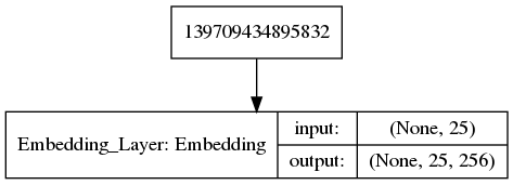
Running which we get:
Layer (type)                 Output Shape              Param #
=================================================================
Embedding_Layer (Embedding)  (None, 25, 256)           262144
=================================================================
Total params: 262,144
Trainable params: 262,144
Non-trainable params: 0
4. Recurrent layers
Recurrent layers are good for data where sequence is important. For example the sequence of words is important to the meaning of a sentence and its classification thereof. And the sequence of image frames is important to classify an action in a video.
Input to recurrent layers is a fixed-length sequence of vectors with each vector representing an element in that sequence. When working with text the elements of the sequence are words and each word represented as a numerical vector either via the embedding layer or externally supplied say with FastText for example. One could also conceive of supplying sequences of image frames from a video where each frame is first converted to a vector via convolution.

The recurrent layer turns this sequence of input vectors into a single output vector of size equal to the number of units employed in the layer. Of its many variations, LSTM and GRU are the most popular implementations of recurrent layers and we focus on them here.
4.1 LSTM
We refer to Colah’s blog for the equations defining the transformations taking place in an LSTM layer. Figure 3 below depicts what an LSTM cell does to incoming input.
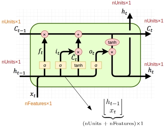
An LSTM cell contains four dense layers (three with sigmoid activation and one with tanh activation) all employing the same number of units specified for the LSTM cell. As shown in Figire 3, each of these dense layers takes the same input that is a concatenation of previous hidden state h_(t-1) and the current input sequence x_t. But they all have their own set of weights and biases that they learn during training. So each will contribute the same number of trainable parameters to the LSTM layer. The following equations describe the transformation of input in an LSTM cell.
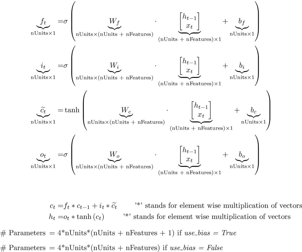
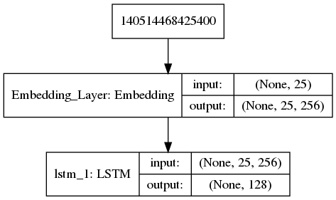
The following code snippet sends in sentences that are at most 25 words long, within an overall vocabulary of 1000 words. The embedding layer turns each word into a 256 long numerical vector, yielding an input of [None, 25, 256] to the LSTM layer with 128 units. Our formula says that the LSTM cell would contribute 4 * 128 * (128 + 256 +1) = 197120 trainable parameters.
nWords = 1000
sequence_length = 25
model = Sequential()
model.add(Embedding(input_dim=nWords, output_dim=256, input_length=sequence_length, name='Embedding_Layer'))
model.add(LSTM(128))
Running the above we see that our formula obtained parameter count matches with what Keras obtains.
Layer (type)                 Output Shape              Param #
=================================================================
Embedding_Layer (Embedding)  (None, 25, 256)           256000
_________________________________________________________________
LSTM_Layer (LSTM)            (None, 128)               197120
=================================================================
Total params: 453,120
Trainable params: 453,120
Non-trainable params: 0
4.2 GRU
Having gone through in some detail over the LSTM cell, we can breeze through the GRU cell as the ideas are similar. The image is all we need to determine how many parameters it adds to the model.
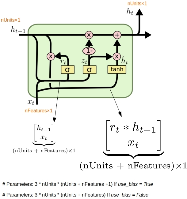
The tanh dense layer has a different input from the other two sigmoid dense layer. But the shape and size of the inputs are identical leading to the above formula. If we run the same piece of code as before with LSTM replaced by GRU as in:
nWords = 1000
sequence_length = 25
model = Sequential()
model.add(Embedding(input_dim=nWords, output_dim=256, input_length=sequence_length, name='Embedding_Layer'))
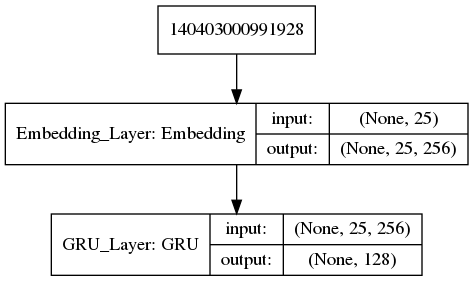
model.add(GRU(128,name='GRU_Layer'))
we ought to get 3 * 128 * (128 + 256 + 1) = 147840 parameters matching with the model summary from Keras below.
_________________________________________________________________
Layer (type)                 Output Shape              Param #
=================================================================
Embedding_Layer (Embedding)  (None, 25, 256)           256000
_________________________________________________________________
GRU_Layer (GRU)              (None, 128)               147840
=================================================================
Total params: 403,840
Trainable params: 403,840
Non-trainable params: 0
5. Summary
We have developed formulae for the number of parameters employed in Dense, Embedding, LSTM and GRU layers in Keras. And we have seen why the input/output tensor shapes make sense given what these layers are expected to do. Here is a summary table.

With that we close this rather short post. We will take up Convolutions and a comprehensive example in the next post in this series.

Pingback: Reconciling Data Shapes and Parameter Counts in Keras – Data Exploration