Sequence Based Text Classification with Convolution Nets

Earlier with the bag of words approach we were getting some really good text classification results. But will that hold, when we take into consideration the sequence of words? There is only one way to find out, let’s get right into the action, where we are doing a head on comparison of traditional approach (Naive Bayes) with a modern neural based one (CNN).

Apparently Feynman once said about the universe, “it’s not complicated, it’s just a lot of it“. A machine might be thinking the same, while dealing with a plethora of words and trying to make sense of relations between them. We use and interpret words or sentences in a context. A lot of context arises from a sequence. Unfortunately, infinitely many sequences of words are possible and most of them are gibberish and yield no context. In our earlier classification articles, we side-stepped this complexity by ignoring the specific sequences of words altogether and instead treating documents as bags of words as per the VSM approach. But looks like there are some new generation models in town (or at least feels like new, even though they have existed for decades) that could account for sequences of words without breaking the bank, and we’re going to see one of those in action today.

Previously, we obtained results from bag of words approach, document vector approach etc. But these techniques don’t emphasize on the sequence of the words and their respective occurrences or relations. Two sentences could have same representation but totally different meaning. Let’s consider one sentence: ‘Thank you for helping me’, now by altering a few words it could be written as, ‘You thank me for helping’. This rearrangement of words though makes a completely new sentence but it’ll be observed as the same when viewed from bag of words approach.

This is where we need such a model which extracts the relation or patterns from a group of words, not from an individual word. In such a scenario, Convolutional Neural Networks (CNN) can produce some really good results. CNNs are known for extracting the patterns from the underlying sentences by focusing on a sequence of words at a time.

Here, we’ll start with a brief CNN introduction and then move on to classification part. As we know CNN is mostly used with the image classification related tasks. So, here we’re taking an example of how a typical convolution neural net works with a 2D image to get some idea about the working of CNN.

1. Convolutional Neural Nets:

CNN i.e. a ‘Convolutional Neural Network’ is a class of deep, feed-forward artificial neural networks, most commonly used for analyzing images. These networks use a variation of multi-layer perceptrons designed to minimal pre-processing.

1.1 CNN Design:

A CNN consists of an input and an output layer, as well as multiple hidden layers. The hidden layers of a CNN typically consist of convolutional layers, pooling layers, fully connected layers and normalization layers (optional).

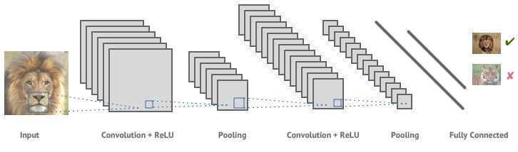
1.2 Convolutional + ReLU:

After receiving the input from the input layer, convolution layer is the first layer to apply operations on the inputted data. This layer applies a convolution operation to the input, and then passes the result to the next layer. This convolution operation is applied with the help of kernel, a kernel is nothing but a set of weights. (The moving window in the picture below is a kernel)

1.3 Pooling:

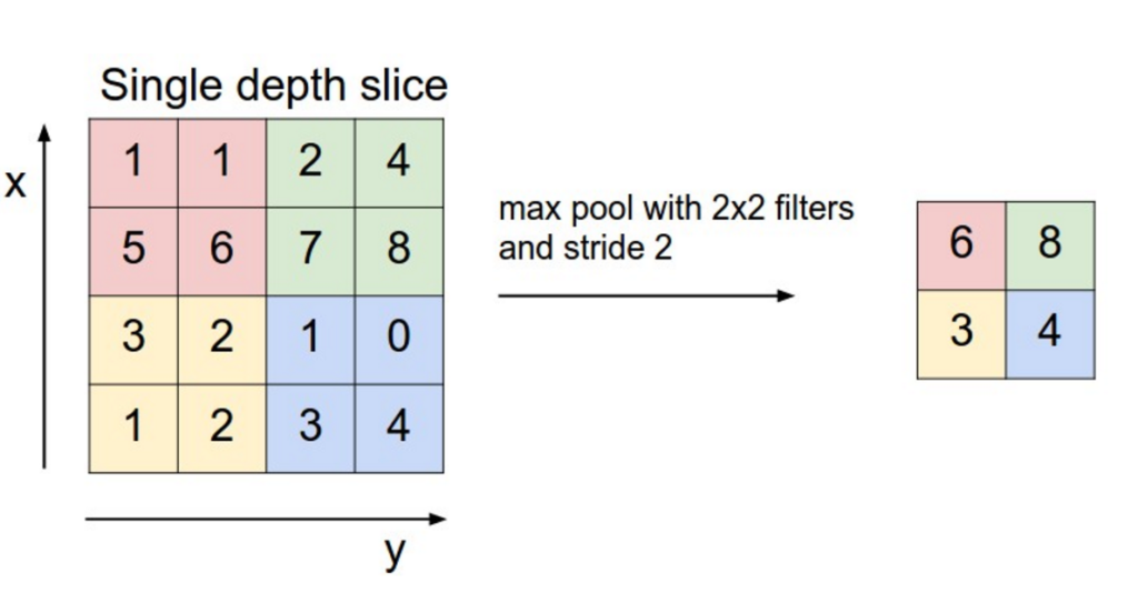
Convolution networks may include local or global pooling layers, which combine the outputs of neuron clusters at one layer into a single neuron in the next layer. Below is the example of max-pooling which simply selects the maximum value from a group.

1.4 Fully Connected:

Fully connected layers takes the final pooling layer and flattens it to obtain the number of neurons and then those number of input values are fed into it.

So, with this post we are trying to classify custom text sequences using CNN and Naive Bayes with tf-idf for comparison. CNN here is implemented with the help of Keras and tensorflow as its back-end. For Naive bayes we are using sklearn or scikit-learn.

2. Implementation:

2.1 Generating custom text data:

We’ll be using the same text corpus which was used in the LSTM article and you can refer it by going to this link: LSTM article.

The reason for choosing such a custom corpus is to demonstrate the difference between bag of words approach with Naive Bayes and sequence based approach with convolution nets.

Now we’ll see how encoding and CNN part are implemented to obtain the final results. You can find the related code snippets by visiting this link on GitHub. The main imports for this task are as follows:

In the code snippet below, we fix some random seeds for tensorflow and numpy so that we can get some reproducible results.

2.2 Encoding:

Use the Keras text processor on all the sentences/sequences so it can generate a word index and encode each sequence (Lines 2-4 below) accordingly. Note that we do not need padding as the length of all our sequences is exactly 15.

2.3 CNN Implementation:

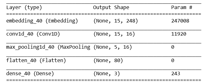
CNN implementation will consist of the embedding layer, convolution layer, pooling layer (we’ll use MaxPooling here), one flatten layer and the final dense layer or the output layer

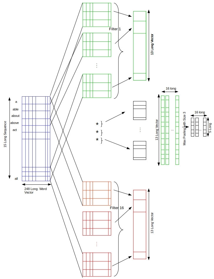
Fifteen words (where each word is a 1-hot vector) in sequence are pumped as the input to an embedding layer that learns the weights for order reduction from 995 long to 248 long numerical vectors. This sequence of 248-long vectors are fed to the first layer of the convolution model i.e. convolutional layer.

• Embedding Layer: The embedding layer from Keras needs the input to be integer encoded, here we are passing our data in 1-hot encoded form. So, here words are represented in form of 1 & 0. Embedding layer will also reduce the overall length of word vector which is initially 995, it’ll be brought down to 248.
• Convolution Layer: The input shape for this layer is (15, 248). And for hyper-parameters, such as number of convolution filters as well as for kernel sizes we have performed multiple simulations and the resulting optimal settings have been used in the final code. Convolution layer performs the extraction of most dominating features or relations from the underlying set of word vectors. This extraction is done with different convolution filters. As they are responsible for extracting different set of features by convolving over the input data. (With the padding=”same” we are getting the output to be (15,16), otherwise it would have been (13,16))
• MaxPooling Layer: These extracted features are then passed to the next layer, which is pooling layer. Here we are using MaxPooling, which means extracting the largest value from the specified window size, which is 3 here. So, from each 3 values of convolution filter output, it’ll select just one largest value. As the input same here was: (15,16). Output shape after selecting just one of each 3 values will be: (5,16). (Keep in mind we’re using padding=”same” here, without this the output would have been (4,16))
• Flatten Layer: Flatten layer is used to convert the output of MaxPooling layer into a vector.
• Dense Layer: This the final output layer with the 3 nodes representing three output classes. It uses softmax as the activation function and generated the probability values as it’s output out of which the node with the maximum value is classified as the final class for that given input.

With the data and model in hand we are ready to train the model and test the predictions. Because this is a multi-class classification we convert the labels to 1-hot vectors, using ‘keras.utils.to_catgegorical‘.

The 80% of the data is split into validation (20% of this 80%, i.e 16% overall) and training sets (64% of the overall data) in multiple training/validation simulations.

• We also using early stopping condition (line 2), which will kick in if the validation loss doesn’t decrease in 5 consecutive epochs.
• We’ll loop over 10 training and validation splits with the help of for loop. The number of epochs can be varied to any number, we will keep it 30 here. As irrespective of number of epochs, training will stop if there is no improvement in validation loss.

2.4 Tf-idf vectors & Naive Bayes Implemetation:

Tf-idf vector generation & Naive Bayes implementation can be followed from LSTM article.

3. Results

3.1 CNN Results

After executing the model, following results are obtained,

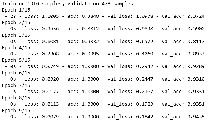
As you can observe with CNN, for some classes we even obtained f1-scores of 0.99 and hence this proves that CNN is really good at performing text classification tasks.

3.2 Naive Bayes results & Comparison:

With the Naive Bayes though the results aren’t that promising, we obtained a f1-score of only 0.23, which is very low as compared to approx 0.95 of CNN.

Figure below shows the f1-score plots of naive bayes and CNN side by side. The diagonal dominance observed here is due to the high f1-scores of CNN.

4. Conclusion:

We worked with a synthetic text corpus designed to exhibit extreme sequence dependent classification targets. And we have seen that pattern recognizing approach such as CNN has done extremely well compared to traditional classifiers working bag-of-words vectors that have no respect for sequence. The result is to be expected and similar to the results obtained with LSTM.

The question is how CNN might do on regular text where we know the sequence of words may not the end all and be all. We will take it up in the next post in this series