In our last article, we were getting some really good results with CNN when we used a custom text corpus. But will CNN manage to hold onto its lead when it competes with SVM in the battle of sentiment analysis, let’s find that out…

“Not all experience the same sentiment while doing the same exact activity”, this quote by Efrat Cybulkiewicz sums up our article’s topic. Today we are going to explore, the sentiment extraction capabilities of Machine & Deep learning models.
In our previous article, we witnessed a head-on comparison between the modern age CNNs and traditional Naive Bayes (NB) model. In that, we used bag of words approach with NB & sequences of data were passed to CNN as input. This time though, the model we are using here from Machine Learning team is, Support Vector Machines (SVM). And from Deep Learning’s corner, we have CNN, which completely decimated NB in it’s previous encounter with a F1-score of well over 0.9 as compared to NB’s 0.3. But the slight advantage CNN held was the data, as it was not real. On the other hand, today we are going with a real-life movie-reviews data-set. So, hold on tight, as our journey of exploring the depths of deep learning is going to start once again.
In this article, we’ll be using the IMDB movies reviews dataset. Our goal will be to classify the reviews in two classes, either positive or negative. To perform the classification, we’ll use convolution neural net which will be backed by Keras and Support vector machine which will be implemented using Scikit-Learn. You can find the complete code of this post by visiting this GitHub repo.
1. About the Text Corpus
We are using movie reviews dataset provided by Stanford. It contains movie reviews from IMDB with their associated binary sentiment polarity labels. It is intended to serve as the benchmark for the sentiment classification. The core dataset contains 50,000 reviews split evenly into 25k train & 25k test reviews (25k positive & 25k negative).
In the entire collection, no more than 30 reviews are allowed for any given movie because reviews for the same movie tend to have correlated ratings. Further, the train and test sets contain a disjoint set of movies, so no significant performance is obtained by memorizing movie-unique terms and their associated with observed labels.
2. Token Generation
Following script can be followed to tokenize the movie reviews.
# Read the Text Corpus, Clean and Tokenize
import numpy as np
from nltk.tokenize import RegexpTokenizer
from nltk.corpus import stopwords
from sklearn.datasets import fetch_20newsgroups
nltk_stopw = stopwords.words('english')

def tokenize (text):        #   no punctuation & starts with a letter & between 2-15 characters in length
    tokens = [word.strip(string.punctuation) for word in RegexpTokenizer(r'\b[a-zA-Z][a-zA-Z0-9]{2,14}\b').tokenize(text)]
    return  [f.lower() for f in tokens if f and f.lower() not in nltk_stopw]

def getMovies():
    X, labels, labelToName  = [], [], { 0 : 'neg', 1: 'pos' }
    for dataset in ['train', 'test']:
        for classIndex, directory in enumerate(['neg', 'pos']):
            dirName = './data/' + dataset + "/" + directory
            for reviewFile in os.listdir(dirName):
                with open (dirName + '/' + reviewFile, 'r') as f:
                    tokens = tokenize (f.read())
                    if (len(tokens) == 0):
                        continue
                X.append(tokens)
                labels.append(classIndex)
    nTokens = [len(x) for x in X]
    return X, np.array(labels), labelToName, nTokens
Here, we have a tokenize function which is responsible for removing all stop words using nltk stop-words as well as retaining words only 3 to 15 characters long.
The other function getMovies is responsible for iterating over the directory containing the ‘pos’ & ‘neg’ data files. After accessing these files, they are passed into the tokenize function to obtain the final tokens. It is also recording the number of tokens in nTokens keyword, which will help us in deciding the sequence length.
3. Preparing Sequences & Vectors
Here, we’ll be using 1D convolutional layers which will take input in form of sequences. Whereas, Support vector machines take tf-idf vectors as input.
3.1 Generating Tf-Idf Vectors
Scikit learn’s tf-idf vectorizer can be used to generate the document vectors and vocabulary from tokens.
# Build Tf-Idf Vectors
from sklearn.feature_extraction.text import TfidfVectorizer
X=np.array([np.array(xi) for xi in X]) # rows:Docs. columns:words
vectorizer = TfidfVectorizer(analyzer=lambda x: x, min_df=1).fit(X)
word_index = vectorizer.vocabulary_
Xencoded = vectorizer.transform(X)
3.2 Getting the Sequences
Using Keras’s text processor we can convert tokens into integers which represent all those words corresponding to their position in the sentence/document. Average length of our documents is close to 200 to we’ll be create sequences for our Conv1D which will be 200 in length. In case, some documents are less than 200 then padding is used to complete it.
import keras
sequenceLength = 200
kTokenizer = keras.preprocessing.text.Tokenizer()
kTokenizer.fit_on_texts(X)
encoded_docs = kTokenizer.texts_to_sequences(X)
Xencoded = keras.preprocessing.sequence.pad_sequences(encoded_docs, maxlen=sequenceLength, padding='post')
4. Implementing Models
Keras will be used with tensorflow as its back-end to implement Convolution neural network whereas we’ll be using sklearn to implement Support vector machine.
Here, 10,000 documents out of 50,000 are put aside for testing purpose which is 20% of the total. And remaining 40,000 will be used as the training data.
from sklearn.model_selection import StratifiedShuffleSplit
sss = StratifiedShuffleSplit(n_splits=1, test_size=0.2, random_state=1).split(Xencoded, labels)
train_indices, test_indices = next(sss)
train_x, test_x = Xencoded[train_indices], Xencoded[test_indices]
4.1 Convolution Neural Net

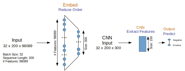
The number of convolution layers used in the model has been kept to minimum (just one), to keep it as simple as possible. Before inputting the sequences into convolution layer, we have a embedding layer which takes 98089 long 1-hot vectors and convert them to 300-long vectors.
early_stop = keras.callbacks.EarlyStopping(monitor='val_loss', min_delta=0, patience=5, verbose=2, mode='auto', restore_best_weights=False)
 model = keras.models.Sequential()
 embedding = keras.layers.embeddings.Embedding(input_dim=len(kTokenizer.word_index)+1, output_dim=300, input_length=sequenceLength, trainable=True)
 model.add(embedding)
 model.add(keras.layers.Conv1D(150, 5, activation='relu', padding='valid'))
 model.add(keras.layers.MaxPooling1D(5, padding = 'valid'))
 model.add(keras.layers.Flatten())
 model.add(keras.layers.Dense(numClasses, activation='softmax'))
 model.compile(optimizer='adam', loss='categorical_crossentropy', metrics=['acc'])
 print(model.summary())
We are also using early stopping condition to stop earlier when there is not much improvement in the validation loss, this also prevents over model from over-fitting. The output labels which are in form of a vector, are then used to obtain the dominating label with the help of argmax.
train_labels = keras.utils.to_categorical(labels[train_indices], len(labelToName))
test_labels = keras.utils.to_categorical(labels[test_indices], len(labelToName))
early_stop = keras.callbacks.EarlyStopping(monitor='val_loss', min_delta=0, patience=5, verbose=2, mode='auto', restore_best_weights=False)
history = model.fit(x=train_x, y=train_labels, epochs=50, batch_size=32, shuffle=True, validation_data = (test_x, test_labels), verbose=2, callbacks=[early_stop])
predicted = model.predict(test_x, verbose=2)
predicted_labels = predicted.argmax(axis=1)
4.2 Support Vector Machine
We’ll use scikit learn to implement SVM here.
from sklearn.svm import LinearSVC
model = LinearSVC(tol=1.0e-6,max_iter=5000,verbose=1)
train_labels = labels[train_indices]
test_labels = labels[test_indices]
model.fit(train_x, train_labels)
predicted_labels = model.predict(test_x)
5. Simulations
In results, we’ll be using Sklearn’s classification report & confusion matrix methods to generate f1-scores and confusion matrix respectively.
# Get Confusion Matrix and Classification Report
from sklearn.metrics import classification_report, confusion_matrix
print (confusion_matrix(labels[test_indices], predicted_labels))
print (classification_report(labels[test_indices], predicted_labels, digits=4, target_names=namesInLabelOrd
5.1 Executing CNN
We’ll use jupyter notebook here to execute Convolution nets. GPU versions of Tensorflow as well as Keras are used.
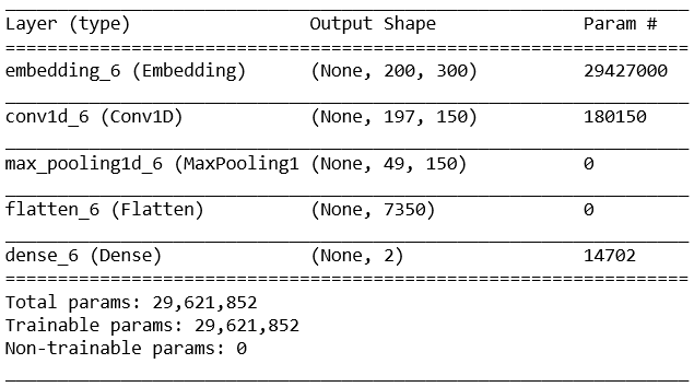
Model Summary for CNN is as follows:

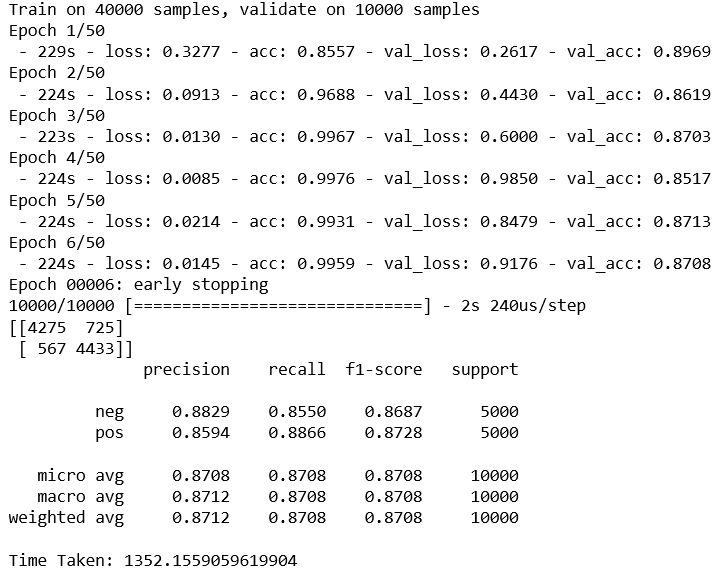
Execution summary for the CNN with early stopping enabled results in,

CUDA enabled Nvidia GPU has been used for the execution of model which means the training part only takes 1/6th of the time taken by a typical CPU.
5.2 SVM Execution
SVM execution takes very less time and results in a f1-score of 0.90. Code for both the models can be obtained from the following github respository link.
6. Conclusion
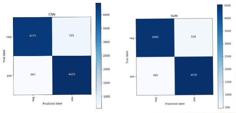
The performance of both the classifiers can be compared through these confusion matrices:

Numbers across the diagonals shows the dominance of both the classifiers in this binary classification of positive & negative sentiments. One advantage with SVM though is that of model training time as it aligned its decision boundaries in a few milli-seconds. Whereas even with GPU, CNN took more than 20 minutes to tune its parameters.
So, this was our sentimental CNN with the IMDB movies review data. In our next post, we will take our journey of deep learning exploration one step further into multi-class classification & word-embeddings.
