Attention as Adaptive Tf-Idf for Deep Learning

Attention is like tf-idf for deep learning. Both attention and tf-idf boost the importance of some words over others. But while tf-idf weight vectors are static for a set of documents, the attention weight vectors will adapt depending on the particular classification objective. Attention derives larger weights for those words that are influencing the classification objective, thus opening a window into the decision making process with in the deep learning blackbox…

Pay attention! So your parents told you right? And good thing too. We may actually learn something when we pay attention. Deep learning is no exception!. By paying attention, a shallow network of layers can perhaps outsmart a large stack of layers for the same prediction task. Or it may need a lot less data to train on, or use fewer parameters for the same skill gained. Much like acing the exams by just paying attention in class, rather than having to slog into the wee hours the night before the exam! All good things and inherently appealing to boot, right?

Tf-idf weighting of words has long been the mainstay in building document vectors for a variety of NLP tasks. But the tf-idf vectors are fixed for a given repository of documents no matter what the classification objective is. But it is quite common to have a text corpus that needs to be classified by different objectives. Perhaps by the nature of their content, i.e. politics/science/sports or perhaps by the places they apply to i.e. America/Asia/Europe or perhaps by sentiment positive/neutral/negative etc…. In each case, the words/phrases that influence the decision making process for the particular classification objective would be naturally different. But the tf-idf vectors are static. So the entire burden is essentially on the classification algorithm to yield different predictions for the same prediction vectors even while the classification objective changes.

Enabling deep learning techniques to advantageously use different weights for different words, and as a function of the NLP task in question is what Attention Mechanism is about. And it is automatic. Attention embeds itself within the overall optimization process and picks out the which words/phrases are driving a particular classification objective. So the final vectors to the prediction step are customized for the objective in question. This extra flexibility allows for better predictive performance.

The purpose of this post is to illustrate the benefits of attention in the context of a simple multi-class, multi-label document classification task. The sequence of words is not relevant for the classification task here. We implement Bahdanau Attention on top of an embedding layer. Functional API in Keras is used when masking is not in place. A custom attention layer from Christos Baziotis is used when masking is needed. Makes no difference for our illustration problem here however. We will go through some code snippets here but the full code can be downloaded from github. Let us get on with it then.

1. Attention to Identify the Important Words

Not all words in a document are important for its classification. We may have an idea for sure. For example the presence of words like good may indicate a positive review of a movie. The phrase not good would indicate a negative review, while not so good may indicate neutral, with so so good going back to positive while so so indicating neutral. You can replace good with bad and reverse the positive and negative classifications. But while terrific may indicate a positive review, not terrific is likely neutral. You get the point. There are practically infinitely many combinations of commonly used words and phrases whose net sentiment can go different ways. Attempting to account for them all with say grep/regex (or even with a full blown search engine using sophisticated boolean logic with phrase slop) would be a fool’s errand. Besides, these influential words will likely be a bit different from one corpus to another. So a painstakingly built script on one corpus will not work on another. This approach will simply not scale.

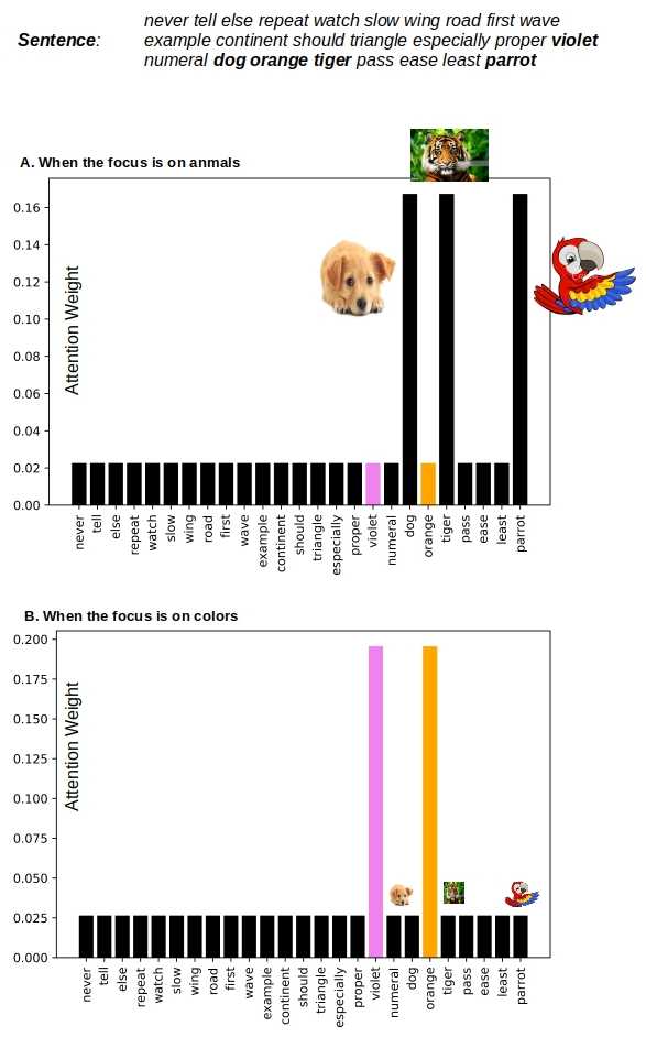
Instead we want a machine to do this for us. Given a training set of documents, we want the algorithm to learn which words and their combinations are driving the indicated classification objective. This is what Attention Mechanism is about in deep learning. It gives the algorithm a means to identify the controlling words and phrases as part of the ongoing classification task. Thus, depending on the classification task different weights for words/sentences are automatically derived for the same sentence/document respectively. Figure 1 below illustrates this for a sentence. The larger attention weights obtained for color (or animal if the objective is to classify by animal reference) words help drive the sentence vector to fall into the correct color (or animal) buckets.

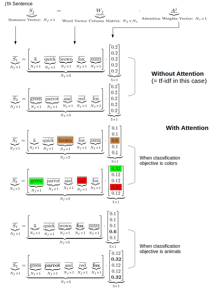
An excellent side benefit also is that we have some insight into why the algorithm placed a document into whatever classes it did. That is huge, as we are talking explainable AI. The word-level attention mechanism implemented here is from the work of Bahdanau et. al. Another excellent reference that extends the idea up the hierarchy for sentence-level attention is due to Yang et. al .

2. Implementing Bahdanau Attention in Keras

A sentence is a sequence of words. Each word is a numerical vector of some length – same length for very word. The numerical vectors for words can be obtained either directly with an embedding layer in Keras or imported into the model from an external source such as FastText. The attention weight vector is obtained as part of the training process following the equations presented in Yang et. al. The equations are straightforward. Here is our naming and indexing convention.

• N_s: The maximum number of words in any sentence
• N_a: Arbitrary/Optional number of units in the first tanh dense layer
• N_f: The length of each word-vector
• w_i: word-vector for the i’th word in the sentence.
• A^j_i: Attention weight for the i’th word in j’th sentence
• S_j: j’th sentence

Each of these N_s word-vectors of a sentence are first put through a tanh dense layer with N_a units (Yang et al choose N_a to be about 100). This is followed by another tanh dense layer with 1 unit. The purpose of the second tanh layer is to reduce the N_a long vector from the first layer to a scalar. We could of course use the just one tanh layer with 1 unit, but having two tanh layers with the first one having N_a > 1 offers more flexibility. Also, instead of a second tanh layer, one could perhaps sum up N_a values in the vector after the first tanh layer to get this scalar – but not tried here. In any case the end result in one scalar value per word in the sentence.

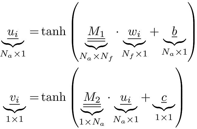
Collecting the v_i above for each word in j’th sentence yields an N_s long vector v which upon softmax gives the N_s long attention weights vector A^j for that sentence. The sentence vector is then obtained as simply the sum of attention weighted word-vectors.

2.1 Without masking

While the equations are straightforward, implementing attention in Keras is a bit tricky. When masking is not used – that is when every sentence has exactly the same number of words, it is a bit easier and we can implement it with the functional API. If we go this route though, all shorter sentences need to be appended with a dummy/unused word (like zzzzz in Figure 1) as many times as needed to make them all as long as the longest sentence. Somewhat inefficient but for simple demo problems like the one in this post it is not an issue. Figure 2 below (modified ideas from Philippe Rémy, and a you-tube video from Shuyi Wang) shows what we need to do implement attention in Keras when masking not used.

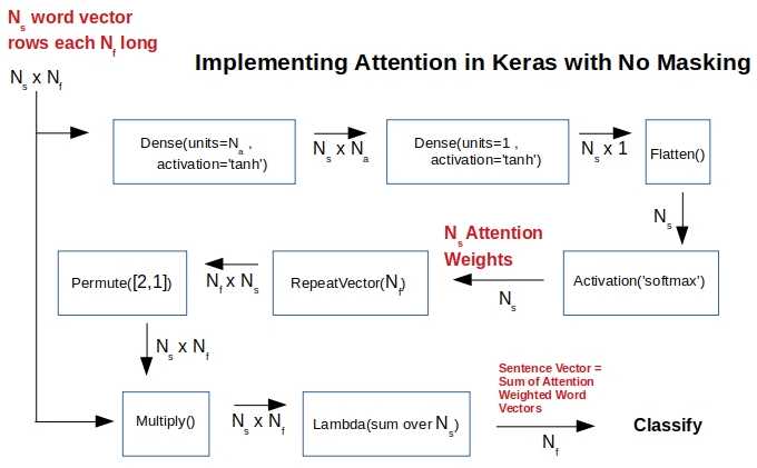
The above can be defined as a function that takes a sequence of word-vectors as argument and returns a sentence vector as per Equation 2.

2.2 With masking

Christos Baziotis has an implementation of attention as a custom layer that supports masking so we do not have to explicitly add dummy words to sentences. We use that implementation in our model when we want to use masking.

For our demo problem it yields the same results as the implementation in Section 2.1 without masking.

3. Example: Multi-Class, Multi-label Classification with Attention

All that is left to do now is to put this to work on a text corpus and show that attention works to dynamically identify the important words given the objective of the NLP task. The code to reproduce the results can be downloaded from github.

Sentences that are 15-25 words in length are generated by randomly picking words from a list of 1000 unique words, including some color & animal words. A sentence may have up to 4 different color words and/or animal words. The objective is to classify the sentences either by color or animal reference they contain. When the objective is to classify by color, a sentence falls into all the color buckets that it contains as words. Likewise when classification objective is by animal reference. Thus, whatever the classification criterion is, we are talking about a multi-class, multi-label classification problem. The snippet of code below generates the documents.

The label vector for a sentence is number_of_colors + 1 long (when classifying by color) with 1 in the location for the color words that are present in the sentence and 0 otherwise. For example we use the 7 rainbow colors VIBGYOR so the length of the label vector is 8 – including the ‘none’ label.

Building the overall Keras model is straightforward. We define an intermediate model so we can output the attention weights out of the layer with the name ‘attention_vector_layer’ . As this is a multi-class, multi-label classification problem we use sigmoid activation in the final dense layer and binary_crossentropy with categorical_accuracy as the metric. Check the article by Tobias Sterbak and discussions on Stackoverflow on why those are the right choices.

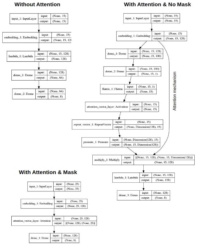
The model is run with/without attention and with/without masking. The tensor flow diagrams produced by Keras confirm our models in Section 2.

4. Results

Simulations with & without attention/masking are run for both when the objective is colors and animals. Thirteen hundred sentences with train/valid/test: 832/208/260 split are used in all the four runs. Whenever the predicted probability for a class is > 0.5 for a sentence, we label that sentence with that class. Figure 3 shows the obtained attention weights for words in one such sentence for the different classification objectives. Definitely what we want to see, as the important words have been automatically picked by the attention mechanism and given larger weights compared to others. This translates directly into larger probabilities for the correct classes for a sentence as these words are driving the classification decision.

For the same sentence Figure 4 below shows the class probabilities. With attention, the probabilities for the correct classes are near 1.0, and the probabilities for the rest are near 0.0. Exactly what we want. Without attention we see that probabilities as large as 0.75 are predicted for the incorrect class indigo, and as low as 0.05 for the correct class tiger.

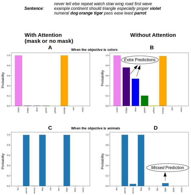
Classification with attention yielded 100% accurate predictions for all the 260 test documents. That is, every actual class and only the actual classes was predicted (probability > 0.5) for every test document. Without attention, some correct classes were missed (predicted probability < 0.5) and some wrong classes were predicted (predicted probability > 0.5) as shown in Figure 4.

5. Conclusions

The attention mechanism enables a model to attach larger weights to words that are important for a given classification task. This enhances the classification accuracy while shedding light on why a particular document is classified into certain buckets – a very useful piece of information for real world applications.

The sequence of words was not relevant for classification in the example here. So there was no need for fancier recurrent or convolutional layers. But sequence of words, and relative proximity of words is important for the meaning conveyed in real documents. In the upcoming posts we will apply the same attention mechanism on top of LSTM (uni or bidirectional with return_sequences=True) layers that can better handle documents where sequence of words is important.