
Convolutional layers and their cousins the pooling layers are examined for shape modification and parameter counts as functions of layer parameters in Keras/Tensorflow…
Keras is synonymous with deep learning. Building multi-input, multi-output network of connected layers is a routine task with Keras. The data/tensors (multidimensional matrix of numbers) twist & turn their way from layer to layer, from entry to exit, as the network racks up millions of parameters along the way. How the data shape morphs as it squeezes through a layer, and how many parameters that layer adds to the network model are of course a function of the layer in question and how that layer has been instantiated in Keras. In the earlier article Flowing Tensors and Heaping Parameters in Deep Learning:
- We looked at the Dense, Embedding, and Recurrent (LSTM/GRU) layers in some detail to understand how and why the data shape changed as it passed through these layers.
- Using the equations describing the data modification within the layer, we derived formulae for the number of trainable parameters used in each of these layers for the said modification.
We continue the exercise here with Convolutional and Pooling layers heavily used in image classification. We close the series by running the Visual question answering model and confirm that our formulae/analysis are correct for the trainable parameters and output shapes. The full code for the snippets can be obtained from github.
1. Convolutional Layer
Convolutional layers are basically feature extractors. They are mostly used with images, but can be applied to text as well for pattern/feature identification and classification thereof. When working with text, we first turn words into numerical vectors using an Embedding layer or using externally supplied vectors.
1.1 Input Shape
Input to a convolutional layer can be batches of images or sentences. Keras default for input data is “channels_last” meaning the number of channels/features N_c would be the last dimension, and as usual the first dimension is the batch_size left out here as ‘None’. In between these two are the dimensions of the image (or the sequence length in case of text).
[batch_size, {dimensions of image/text}, Number of channels/features]

1.2 Output Shape
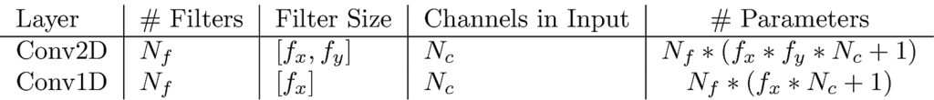
The convolution operation is well explained with pretty pictures and such in a number of articles. Our interest here is in shape transformation and parameter counts. Figure 2 and Table 1 below summarize the discussion that follows for shape transformations.

- The output of convolutional layer is produced by filters. Each filter has a size like [f_x, f_y] for example in 2-d. Each filter is automatically N_c deep where N_c is the number of channels in the input. That is, its actual shape is [f_x, f_y, N_c]
- Each filter generates a new channel for the output. That is, convolving an image with however many channels with 64 filters yields an output image with 64 channels.
- The size [O_x, O_y] of the output image above in 2 depends on two settings in Keras.
- strides s_x, s_y: How the filter moves along the input matrix of numbers/pixels for its element-wise product and summation operation. s=1 means that the filter moves one pixel/cell at a time
- padding: When the filter dimensions (f_x and f_y) and its strides (s_x and s_y) across the image (I_x and I_y) are not exactly right, a part of the input data may not get processed by the convolutional layer. This is what happens by default (padding=valid) in Keras. When padding is set to same, the input image/matrix is padded around with fake data like 0, just so all the real data does get processed by the filter. Table 1 below summarizes the shape and size of the output image upon convolution in Keras with Tensorflow.

1.3 Parameter Counts
Besides adding to the number of channels in the output image, each filter brings a bunch of parameters to the table. We have seen that a filter has the shape [f_x, f_y, N_c] in 2-d (or [f_x, N_c] in 1-d image/text) where N_c is the number of channels in the input. The key properties when it comes to filter parameters are as follows.
- Even as a filter strides and slides convolving across the input image/matrix, it uses the same parameters.
- There is one weight associated with each filter cell and channel. In other words a filter has f_x * f_y * N_c weights.
- The entire filter has one bias parameter.
So if a convolutional layer employs N_f filters each of size [f_x, f_y] convolving over an input image with N_c channels the following equation gives the number of parameters added to the model.
1.4 Example
Consider the following snippet of code where 100×95 size ‘rgb’ images are put through two convolutional layers in series.
model = Sequential()
model.add(Conv2D(filters=55, kernel_size=(3, 2), padding="valid", strides=(2, 1), input_shape=(100, 95, 3)))
model.add(Conv2D(filters=35, kernel_size=(5, 2), padding="same", strides=(3, 2)))
Putting our formulae from Table 1 and Equation 1 to work, we should expect to get the following output shapes and parameter counts.
| O_x | O_y | # Params | |
| 1 | ceil((100-3+1)/2)=49 | ceil((95-2+1)/1) =94 | 55 * (3*2*3+1)=1045 |
| 2 | ceiling(49/3) = 17 | ceiling(94/2) = 47 | 35*(5*2*55+1) =19285 |
The output below upon running Keras matches with our predictions.
Layer (type)                 Output Shape              Param #
=================================================================
Conv_Layer_1 (Conv2D)        (None, 49, 94, 55)        1045
_________________________________________________________________
Conv_Layer_2 (Conv2D)        (None, 17, 47, 35)        19285
=================================================================
Total params: 20,330
Trainable params: 20,330
Non-trainable params: 0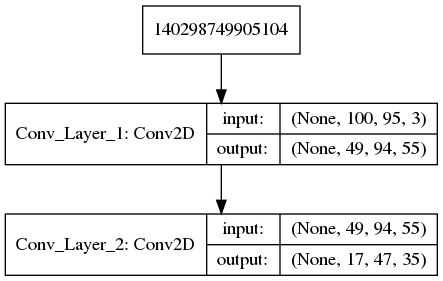
2. Pooling Layer
Pooling layers work hand-in-hand with convolution layers. Their purpose is to reduce the dimensions of the image output by an upstream convolutional layer. They do it by picking a single (average or max for example) from each pooling zone. Pooling zone is a patch of area (much like a filter in the convolutional layer) that moves around the input image as per the settings for strides and padding. Here are key points about pooling layers.
- Input/Output Shapes: The rules/formulae for computing the output image size (O_x, O_y) are identical to that for convolutional layers. The parameter pooling_size serves the role of kernel_size used in defining the filters for convolutional layers. Also, unless separately specified, strides is taken to be the same as pooling_size. So we simply refer to Table 1.
- Trainable Parameters: There are no parameters.
All that a pooling layer does is to apply fixed rules for data/shape transformation. Here is the same example as in Section 1.4 but with pooling layer employed.
model = Sequential()
model.add(MaxPooling2D(pool_size=(3, 2), padding="valid", strides=(2, 1),input_shape=(100, 95, 3),name='Valid_Pool_Layer'))
model.add(MaxPooling2D(pool_size=(5, 2), padding="same", strides=(3, 2),name='Same_Pool_Layer'))
Running which we get the output image shapes (O_x and O_y) to be identical to what we saw earlier with convolution layers. Pooling occurs in all N_c channels independently so the number of channels are preserved.
Layer (type)                 Output Shape              Param #
=================================================================
Valid_Pool_Layer_1 (MaxPooli (None, 49, 94, 3)         0
_________________________________________________________________
Same_Pool_Layer_2 (MaxPoolin (None, 17, 47, 3)         0
=================================================================
Total params: 0
Trainable params: 0
Non-trainable params: 0
3. Visual question answering model
We wrap up this post by putting our formulae to work on the example problem in Keras Guide. Among other layers, the example uses the Dense, Embedding, LSTM, Conv2D and Pooling layers that we have studied in this series. Here is the quote from their description:
This model can select the correct one-word answer when asked a natural-language question about a picture.
It works by encoding the question into a vector, encoding the image into a vector, concatenating the two, and training on top a logistic regression over some vocabulary of potential answers.
Keras Guide
Here is a summary of our formulae including the ones from the previous article. We will refer to it in our verification.

The default settings in Keras for various layers need to be noted.
- Convolution Layers: strides=(1,1), padding=’valid’
- Pooling Layers: strides = pool_size, padding=’valid’
- Dense, LSTM Layers: use_bias = True
The code snippets, the expected shapes/parameter-counts as per our formulae and the actual Keras output upon, and are shown below for each layer in that order.
_________________________________________________________________
Layer (type)                 Output Shape              Param #
=================================================================
vision_model.add(Conv2D(64, (3, 3), activation='relu', padding='same', input_shape=(224, 224, 3))) # Code snippet

O_x = O_y = ceil(224/1) = 224	# As per formulae in Figure 5
Num. Params: 64 * (3 * 3 * 3 + 1) = 64*28 = 1792	#	As per formulae in Figure 5

conv2d_1 (Conv2D)		(None, 224, 224, 64)		1792	# Actual by Keras/Tensorflow
_________________________________________________________________
vision_model.add(Conv2D(64, (3, 3), activation='relu'))

O_x = O_y = ceil((224 - 3 + 1)/1) = 222
Num. Params: 64 * (3*3*64 +1) = 64 * 577 = 36928

conv2d_2 (Conv2D)            (None, 222, 222, 64)      36928
_________________________________________________________________
vision_model.add(MaxPooling2D((2, 2)))

O_x = O_y = ceil((222 - 2 + 1)/2) = 111
Num. Params: 0

max_pooling2d_1 (MaxPooling2 (None, 111, 111, 64)      0
_________________________________________________________________
vision_model.add(Conv2D(128, (3, 3), activation='relu', padding='same'))

O_x = O_y = ceil(111/1) = 111
Num. Params: 128 * (3 * 3 * 64 + 1) = 73856

conv2d_3 (Conv2D)            (None, 111, 111, 128)     73856
_________________________________________________________________
vision_model.add(Conv2D(128, (3, 3), activation='relu'))

O_x = O_y = ceil((111 - 3 + 1)/1) = 109
Num. Params: 128 * (3 * 3 * 128 + 1) = 147584

conv2d_4 (Conv2D)            (None, 109, 109, 128)     147584
_________________________________________________________________
vision_model.add(MaxPooling2D((2, 2)))

O_x = O_y = ceil((109 - 2 + 1)/2) = 54
Num. Params: 0

max_pooling2d_2 (MaxPooling2 (None, 54, 54, 128)       0
_________________________________________________________________
vision_model.add(Conv2D(256, (3, 3), activation='relu', padding='same'))

O_x = O_y = ceil(54/1) = 54
Num. Params: 256 * (3 * 3 * 128 + 1) = 295168

conv2d_5 (Conv2D)            (None, 54, 54, 256)       295168
_________________________________________________________________
vision_model.add(Conv2D(256, (3, 3), activation='relu'))

O_x = O_y = ceil((54-3+1)/1) = 52
Num. Params: 256 * (3 * 3 * 256 + 1) = 590080

conv2d_6 (Conv2D)            (None, 52, 52, 256)       590080
_________________________________________________________________
vision_model.add(Conv2D(256, (3, 3), activation='relu'))

O_x = O_y = ceil((52-3+1)/1) = 50
Num. Params: 256 * (3 * 3 * 256 + 1) = 590080

conv2d_7 (Conv2D)            (None, 50, 50, 256)       590080
_________________________________________________________________
vision_model.add(MaxPooling2D((2, 2)))

O_x = O_y = ceil((50 - 2 + 1)/2) = 25
Num. Params: 0

max_pooling2d_3 (MaxPooling2 (None, 25, 25, 256)       0
_________________________________________________________________
vision_model.add(Flatten())

All data as a single vector of size: 25*25*256 = 160000
Num. Params = 0

flatten_1 (Flatten)          (None, 160000)            0
=================================================================
Total params: 1,735,488
Trainable params: 1,735,488
Non-trainable params: 0
_________________________________________________________________
__________________________________________________________________________________________________


encoded_image = vision_model(image_input)


Layer (type)                    Output Shape         Param #     Connected to
==================================================================================================
question_input = Input(shape=(100,), dtype='int32')

sequenceLength = 100
Num. Params = 0

input_2 (InputLayer)            (None, 100)          0
__________________________________________________________________________________________________
embedded_question = Embedding(input_dim=10000, output_dim=256, input_length=100)(question_input)

nWords = 10000
Num. Params = size of weight matrix = nWords * output_dim = 10000 * 256 = 2560000

embedding_1 (Embedding)         (None, 100, 256)     2560000     input_2[0][0]
__________________________________________________________________________________________________
input_1 (InputLayer)            (None, 224, 224, 3)  0
__________________________________________________________________________________________________
encoded_question = LSTM(256)(embedded_question)

nFeatures=256, nUunits=256
Num. Params = 4*nUnits*(nUnits+nFeatures+1) = 4*256*513 = 525312

lstm_1 (LSTM)                   (None, 256)          525312      embedding_1[0][0]
__________________________________________________________________________________________________
(this is just the convolved image as a vector obtained above after 'flatten_1')
sequential_1 (Sequential)       (None, 160000)       1735488     input_1[0][0]
__________________________________________________________________________________________________
merged = keras.layers.concatenate([encoded_question, encoded_image])

Output size: 256 (from question/LSTM) + 160000 (from image/Conv2D) = 160256
Num. Params = 0

concatenate_1 (Concatenate)     (None, 160256)       0           lstm_1[0][0]
                                                                 sequential_1[1][0]
__________________________________________________________________________________________________
output = Dense(1000, activation='softmax')(merged)

nFeatures = 160256, nUnits=1000, Output size: 1000
#Params = nUnits*(nFeatures+1) = 1000 * (160256 + 1) = 160257000

dense_1 (Dense)                 (None, 1000)         160257000   concatenate_1[0][0]
==================================================================================================
Total params: 165,077,800
Trainable params: 165,077,800
Non-trainable params: 0
We note with satisfaction that our predictions for the output shape and the number of trainable parameters matches exactly with Keras gets for each and every layer as the data moves from input to output.
4. Conclusions
In this series we have gone under the hood of some popular layers to see how they twist the incoming data shapes and how many parameters they employ. Understanding these machinations from the fundamentals removes the mystery behind it all and enables us to design efficient models for new applications.