
Sequence respecting approaches have an edge over bag-of-words implementations when the said sequence is material to classification. Long Short Term Memory (LSTM) neural nets with word sequences are evaluated against Naive Bayes with tf-idf vectors on a synthetic text corpus for classification effectiveness.
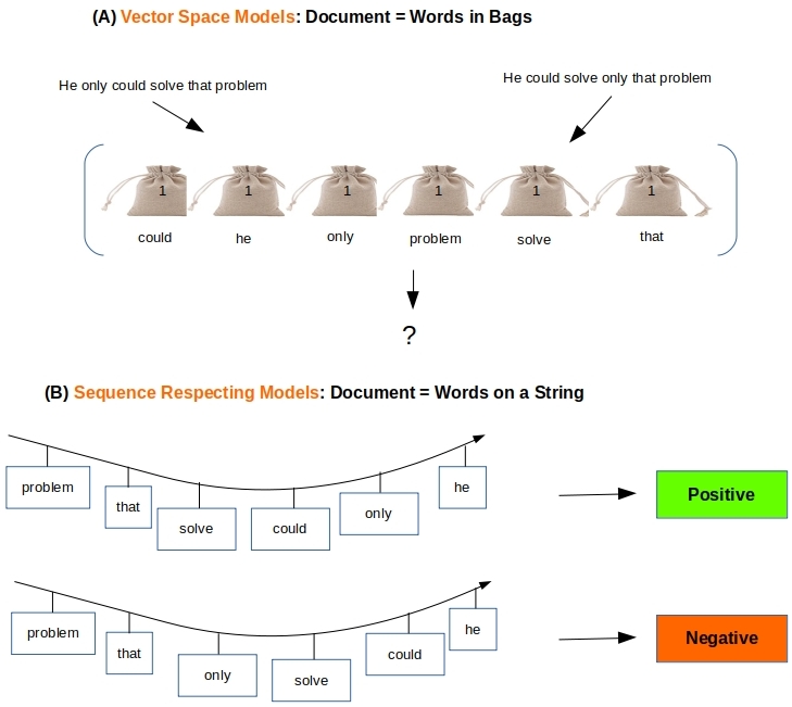
Consider the two one-liners: “Eat to Live” and “Live to Eat“. They contain the same words, but in different order – leading to a big difference in meaning. Bag of words based models cannot tell these documents apart and so place them in the same cluster or classification bucket. Word-embeddings are of no help either as the pre-trained or custom word vectors are a function of the word alone, without any consideration to the position of that word in a sentence. All the NLP exercises we have considered in the earlier posts (classification, clustering) have used this bag-of-words approach to turn documents into numerical vectors (with or without word-embeddings) and hence suffer the same deficiency. This is where the promise of deep learning with Long Short-Term Memory (LSTM) neural networks can be put to test.
LSTM neural nets are an offshoot of Recurrent Neural Nets (RNN) whose hall mark is learning & predicting from sequences – such as sentences/speech that are sequences of words, or monitoring data that evolves with time. LSTM neural nets remedy some short comings associated with learning from long sequences and so are more efficient compared to RNN. There is a lot that has been written about RNN and LSTM networks so we will not delve into the details here. See Karpathy’s article, Colah’s blog for an excellent introduction to RNNs, LSTMs, and what they can do. And of course any number of articles on Medium and those written by Jason Brownlee at Machine Learning Mastery.
This post attempts to classify synthetic word sequences with LSTM and with Naive Bayes using tf-idf vectors. LSTM is implemented via Keras with Tensorflow backend. Naive Bayes is implemented via SciKit. While we go through some code snippets here, the full code for reproducing the results can be downloaded from github. The main imports are as follows.
import numpy as np
import os
import json
from sklearn.metrics import classification_report, confusion_matrix
from sklearn.model_selection import StratifiedShuffleSplit
import random as rn
import keras
import tensorflow as tf
os.environ['TF_CPP_MIN_LOG_LEVEL']='2'
In the code snippet below, we fix the random seeds for numpy and tensorflow so we can get reproducible results. Besides, we set PYTHONHASHSEED=0 as an environment variable in the shell before running the simulations.
#All this for reproducibility
np.random.seed(1)
rn.seed(1)
tf.set_random_seed(1)
session_conf = tf.ConfigProto(intra_op_parallelism_threads=1,inter_op_parallelism_threads=1)
sess = tf.Session(graph=tf.get_default_graph(), config=session_conf)
keras.backend.set_session(sess)
1. Construct a Text Corpus
This post is for illustrative puposes. We want to drive home the point that bag-of-words based classifiers fail badly when faced with having to classify text where the sequence of words is the chief differentiator among the classes as seen in Figure 1 above. In order to do that easily we construct a text corpus without worrying about the meaning of the constructed sentences.
# Build the corpus and sequences
with open ('words.txt' , 'r') as f:
  words = sorted(list(set(f.read().lower().strip().split(','))))
X, labels = [], []
labelToName = { 0 : 'ordered', 1 : 'unordered', 2 : 'reversed' }
namesInLabelOrder = ['ordered', 'unordered', 'reversed']
nWords = len(words)
sequenceLength=15
for i in range(0, nWords-sequenceLength):
  X.append(words[i:i+sequenceLength])
  labels.append(0)
for i in range(nWords-sequenceLength, nWords):
  X.append(words[i:nWords] + words[0:sequenceLength + i -nWords])
  labels.append(0)
nSegments = len(X)
for i in range(nSegments):
  X.append(X[i][::-1])
  labels.append(1)
for i in range(nSegments):
  randIndices = np.random.randint(0, size=sequenceLength, high=nWords)
  X.append(list( words[i] for i in randIndices ))
  labels.append(2)
sss = StratifiedShuffleSplit(n_splits=1, test_size=0.2, random_state=1).split(X, labels)
train_indices, test_indices = next(sss)- Pick a set of words like the top 1000 most common words and sort them. Get 995 unique words. Lines 2-6
- Make 3 separate classes of sentences from these words.
- ordered: Take 15 words in a sequence like 0..14, 1..15, … 995..13 etc… from this list. We get 995 such sentences that belong to this ordered class. Lines 9-14
- reversed: Each one of the above sequences is reversed. Lines 16-18
- unordered:Pick 25 words at random to form a sequence. Again 995 such sequences, so all three classes are balanced. Lines 19-22
- Shuffle, and split to get the train & test data sets. We set aside 20% of all the data to be used exclusively for testing. Lines 23-24
The table below shows sample sequences formed by this means and the classes they belong to.
| ordered | reversed | unordered |
| [‘a’, ‘able’, ‘about’, ‘above’, ‘act’, ‘add’, ‘afraid’, ‘after’, ‘again’, ‘against’, ‘age’, ‘ago’, ‘agree’, ‘air’, ‘all’] | [‘all’, ‘air’, ‘agree’, ‘ago’, ‘age’, ‘against’, ‘again’, ‘after’, ‘afraid’, ‘add’, ‘act’, ‘above’, ‘about’, ‘able’, ‘a’] | [‘atom’, ‘ease’, ‘try’, ‘boat’, ‘sleep’, ‘trouble’, ‘see’, ‘push’, ‘take’, ‘who’, ‘cold’, ‘choose’, ‘winter’, ‘own’, ‘side’] |
| [‘able’, ‘about’, ‘above’, ‘act’, ‘add’, ‘afraid’, ‘after’, ‘again’, ‘against’, ‘age’, ‘ago’, ‘agree’, ‘air’, ‘all’, ‘allow’] | [‘allow’, ‘all’, ‘air’, ‘agree’, ‘ago’, ‘age’, ‘against’, ‘again’, ‘after’, ‘afraid’, ‘add’, ‘act’, ‘above’, ‘about’, ‘able’] | [‘miss’, ‘hour’, ‘fear’, ‘crop’, ‘farm’, ‘especially’, ‘had’, ‘under’, ‘lost’, ‘true’, ‘equal’, ‘me’, ‘red’, ‘very’, ‘i’] |
| [‘young’, ‘a’, ‘able’, ‘about’, ‘above’, ‘act’, ‘add’, ‘afraid’, ‘after’, ‘again’, ‘against’, ‘age’, ‘ago’, ‘agree’, ‘air’] | [‘air’, ‘agree’, ‘ago’, ‘age’, ‘against’, ‘again’, ‘after’, ‘afraid’, ‘add’, ‘act’, ‘above’, ‘about’, ‘able’, ‘a’, ‘young’] | [‘wing’, ‘mouth’, ‘special’, ‘plane’, ‘person’, ‘pattern’, ‘design’, ‘water’, ‘moon’, ‘happy’, ‘chart’, ‘contain’, ‘leg’, ‘system’, ‘count’] |
2. Document = String of Words
With each document as a string of words we build the data structures that can be consumed as input by various sequence respecting models such as RNN, LSTM etc… in the Keras library.
2.1 Encoding
Use the Keras text processor on all the sentences/sequences so it can generate a word index and encode each sequence (Lines 2-4 below) accordingly. Note that we do not need padding as the length of all our sequences is exactly 15.
# Encode the documents
kTokenizer = keras.preprocessing.text.Tokenizer()
kTokenizer.fit_on_texts(X)
Xencoded = np.array([np.array(xi) for xi in kTokenizer.texts_to_sequences(X)])
labels = np.array(labels)
2.2 LSTM Implementation
We use the most simple LSTM model with an embedding layer, LSTM layer and an output layer illustrated in Figure 2 below.
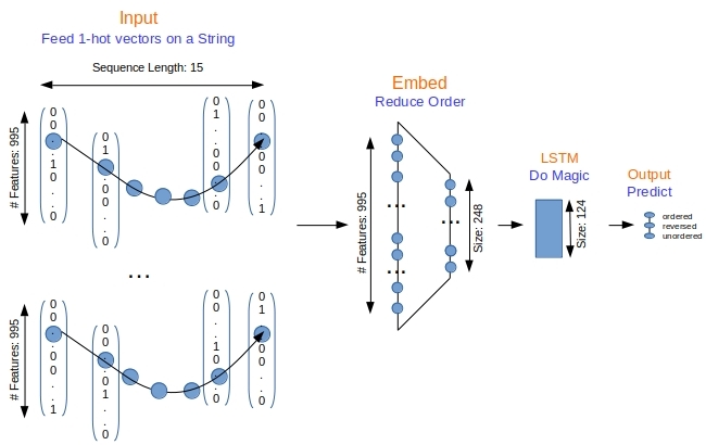
Fifteen words (where each word is a 1-hot vector) in sequence are pumped as the input to an embedding layer that learns the weights for order reduction from 995 long to 248 long numerical vectors. This sequence of 248-long vectors are fed to the LSTM layer to do its magic activating the output layer to yield 3-long numerical vector via softmax. The index of the largest value is then the predicted class
# Build the LSTM model
def getModel():
    units1, units2 = int (nWords/4), int (nWords/8)
    model = keras.models.Sequential()
    model.add(keras.layers.embeddings.Embedding(input_dim = len(kTokenizer.word_index)+1,output_dim=units1,input_length=sequenceLength, trainable=True))
    model.add(keras.layers.LSTM(units = units2, return_sequences =False))
    model.add(keras.layers.Dense(len(labelToName), activation ='softmax'))
    model.compile(optimizer='adam', loss = 'categorical_crossentropy', metrics=['acc'])
return model- Line # 5: The embedding layer builds a word-vector that is 1/4 th size of the input vector. That is, in our case the LSTM layer is fed a numerical vector of size about 250 as our input vector is about 1000 in size.
- Line #6: The LSTM layer outputs a 125 long vector that gets fed to the final layer with softmax activation.
- Line # 7: The final output layer yields a vector that is as long as the number of labels, and the argmax of that vector is the predicted class label.
With the data and model in hand we are ready to train the model and test the predictions. Because this is a multi-class classification we convert the labels to 1-hot vectors in Lines 3-4.
train_x = Xencoded[train_indices]
test_x = Xencoded[test_indices]
train_labels = keras.utils.to_categorical(labels[train_indices], len(labelToName))
test_labels = keras.utils.to_categorical(labels[test_indices], len(labelToName))
The 80% of the data is split into validation (20% of this 80%, i.e 16% overall) and training sets (64% of the overall data) in multiple training/validation simulations.
# Train and test over multiple train/validation sets
early_stop = keras.callbacks.EarlyStopping(monitor='val_loss', min_delta=0, patience=5, verbose=2, mode='auto', restore_best_weights=False)
sss2 = StratifiedShuffleSplit(n_splits=10, test_size=0.2, random_state=1).split(train_x, train_labels)
for i in range(10):
    train_indices_2, val_indices = next(sss2)
    model = getModel()
    model.fit(x=train_x[train_indices_2], y=train_labels[train_indices_2], epochs=50, batch_size=32, shuffle=True, validation_data = (train_x[val_indices], train_labels[val_indices]), verbose=2, callbacks=[early_stop])
    test_loss, test_accuracy = model.evaluate(test_x, test_labels, verbose=2)
    print (test_loss, test_accuracy)
    predicted = model.predict(test_x, verbose=2)
    predicted_labels = predicted.argmax(axis=1)
    print (confusion_matrix(labels[test_indices], predicted_labels))
print (classification_report(labels[test_indices], predicted_labels, digits=4, target_names=namesInLabelOrder))- Line #2: If the validation loss does not decrease in any 5 consecutive epochs, we bail out and stop training.
- Line #3: We set up 10 different train/validation splits to loop over.
- Line #7: Training is done in batches of 32 sentences, and for a maximum of 50 epochs, with early stopping callback in place as discussed.
- Line #11. Get the actual predicted labels from the softmax output vectors.
3. Document = Bags of Words
Building vectors out of bags-of-words approach is straightforward with SciKit’s vectorizers. We have done this many times in the earlier posts. Here we use the tf-idf vectorizer for encoding.
3.1 Encoding
from sklearn.feature_extraction.text import TfidfVectorizer
vectorizer = TfidfVectorizer(analyzer=lambda x: x, min_df=1).fit(X)
Xencoded=vectorizer.transform(X)
The result from Line #2 above is an array of sparse tf-idf numerical vectors that can be fed to any number of traditional classifiers such as Naive Bayes, Support Vector Machines etc… Here we pick Naive Bayes, the simplest of them all.
3.2 Naive Bayes Implementation
We use SciKit’s API for this in the code snippet below. The same training/test data used with LSTM is employed here for training and prediction.
from sklearn.naive_bayes import MultinomialNB
model = MultinomialNB()
train_x = Xencoded[train_indices]
test_x = Xencoded[test_indices]
train_labels = labels[train_indices]
test_labels = labels[test_indices]
model.fit(train_x, train_labels)
predicted_labels = model.predict(test_x)
print (confusion_matrix(labels[test_indices], predicted_labels))
print (classification_report(labels[test_indices], predicted_labels, digits=4, target_names=namesInLabelOrder))
4. Results
The entire code is on github for download as lstm.py and nb.py for the two approaches we are contrasting here.
4.1 LSTM
A sample run with
#!/bin/bash
PYTHONHASHSEED=0 ; pipenv run python lstm.py
yieds:
Layer (type) Output Shape Param #
=================================================================
embedding_1 (Embedding) (None, 15, 248) 247008
_________________________________________________________________
lstm_1 (LSTM) (None, 124) 185008
_________________________________________________________________
dense_1 (Dense) (None, 3) 375
=================================================================
Total params: 432,391
Trainable params: 432,391
Non-trainable params: 0
_________________________________________________________________
None
Train on 1910 samples, validate on 478 samples
Epoch 1/50
- 3s - loss: 1.1036 - acc: 0.2890 - val_loss: 1.1027 - val_acc: 0.2322
Epoch 2/50
- 3s - loss: 1.0813 - acc: 0.4429 - val_loss: 1.1533 - val_acc: 0.2343
Epoch 3/50
..
..
Epoch 11/50
- 3s - loss: 8.5663e-04 - acc: 1.0000 - val_loss: 0.6081 - val_acc: 0.9079
Epoch 00011: early stopping
Confusion Matrix:
[[190 4 5]
[ 0 199 0]
[ 14 28 157]]
Classification Report:
precision recall f1-score support
ordered 0.9314 0.9548 0.9429 199
reversed 0.8615 1.0000 0.9256 199
unordered 0.9691 0.7889 0.8698 199
micro avg 0.9146 0.9146 0.9146 597
macro avg 0.9207 0.9146 0.9128 597
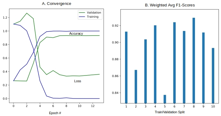
weighted avg 0.9207 0.9146 0.9128 59showing that early stop was triggered in the 11th epoch while getting a f1-score of 0.91. The rate of convergence for a sample split, and the f1-scores obtained with the ten different splits are shown in Figure 3 below.
4.2 Naive Bayes
Running naive bayes is likewise similar, with PYTHONHASHSEED=0 ; pipenv run python nb.py. This yields an average f1-score of 0.23 unfortunately as we see below. This is a far cry from 0.9 obtained with LSTM.
Confusion Matrix:

[[ 36 103  60]
 [ 92  39  68]
 [ 62  75  62]]

Classification Report:

              precision    recall  f1-score   support

     ordered     0.1895    0.1809    0.1851       199
    reversed     0.1797    0.1960    0.1875       199
   unordered     0.3263    0.3116    0.3188       199

   micro avg     0.2295    0.2295    0.2295       597
   macro avg     0.2318    0.2295    0.2305       597
weighted avg     0.2318    0.2295    0.2305       597
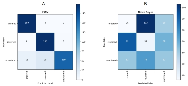
Figure 4 lays out the confusion matrix obtained with LSTM and Naive Bayes side-by-side for comparison. The diagonal dominance in the case of LSTM is indicative of its better predictions and large f1-scores compared to Naive Bayes.
5. Conclusions and Next Steps
That concludes our demonstration that sequence respecting approaches will do better at NLP tasks when the said sequence is material to the task at hand. Thus a string of words approach for documents has advantages over the traditional bag of words approach for the same when the sequence of words is significant. Deep learning models such as LSTM respect the sequence of words and hence can be expected to do better. We constructed a synthetic text corpus and showed that LSTM achieved over 90% for a 3-class f1-score while Naive Bayes classifier working with tf-idf vectors yielded only 0.23.
The artificial nature of the text corpus is the reason for the extreme under performance of Naive Bayes compared to LSTM. But as we said the purpose of this post is illustrative, i.e highlight when & why sequence respecting approaches hold an edge over the traditional bag-of-words approaches. In the next post in this series we will repeat these tests against some real text corpus and see where we stand.
Pingback: BoW to BERT – Data Science Austria